Support Vector Machine
Support Vector Machine (SVM) is a supervised learning algorithm mainly used for classification and regression problems.
The core idea of SVM is to find an optimal hyperplane that separates data of different classes. This hyperplane must not only correctly classify the data, but also maximize the margin between the two classes.
Hyperplane:
- In two-dimensional space, the hyperplane is a straight line.
- In three-dimensional space, the hyperplane is a plane.
- In higher-dimensional space, the hyperplane is a hyperplane that divides the space.
Support Vectors:
- Support vectors are the sample points closest to the hyperplane. These support vectors are crucial for defining the hyperplane.
- SVM selects the optimal hyperplane by maximizing the distance from support vectors to the hyperplane (i.e., maximizing the margin).
Maximum Margin:
- The goal of SVM is to maximize the classification margin, keeping the decision boundary as far away from the two classes of data points as possible. This can effectively reduce the model's generalization error.
Kernel Trick:
- For non-linearly separable data, SVM uses kernel functions to map the data to a higher-dimensional space, in which the data may be linearly separable.
- Commonly used kernel functions include: linear kernel, polynomial kernel, radial basis function (RBF) kernel, etc.
SVM Classification Process
- Select a hyperplane: Find a hyperplane that maximizes the classification margin.
- Train support vectors: Through the SVM algorithm, select the sample points closest to the hyperplane as support vectors.
- Find the optimal hyperplane by maximizing the margin: Select an optimal hyperplane that maximizes the margin.
- Use kernel functions to handle non-linear problems: Map data to a high-dimensional space using kernel functions to solve non-linear separability problems.
Implementing SVM with Python
Next, we will use Python'sscikit-learnlibrary to implement a simple SVM classifier.
1. Install Required Libraries
First, make sure you have installed thescikit-learnlibrary. If not installed, you can use the following command to install it:
pip install scikit-learn
2. Import Libraries
Example
import numpy as np
import matplotlib.pyplot as plt
from sklearn import svm, datasets
from sklearn.model_selection import train_test_split
from sklearn.metrics import accuracy_score
import matplotlib.pyplot as plt
from sklearn import svm, datasets
from sklearn.model_selection import train_test_split
from sklearn.metrics import accuracy_score
3. Load Dataset
We will use thescikit-learnbuilt-in Iris dataset.
Example
# Load the Iris dataset
iris = datasets.load_iris()
X = iris.data[:, :2] # Use only the first two features
y = iris.target
iris = datasets.load_iris()
X = iris.data[:, :2] # Use only the first two features
y = iris.target
4. Split Training and Test Sets
Example
# Split the dataset into training and test sets
X_train, X_test, y_train, y_test = train_test_split(X, y, test_size=0.3, random_state=42)
X_train, X_test, y_train, y_test = train_test_split(X, y, test_size=0.3, random_state=42)
5. Train SVM Model
Example
# Create SVM classifier
clf = svm.SVC(kernel='linear') # Use linear kernel function
# Train the model
clf.fit(X_train, y_train)
clf = svm.SVC(kernel='linear') # Use linear kernel function
# Train the model
clf.fit(X_train, y_train)
6. Prediction and Evaluation
Example
# Make predictions on the test set
y_pred = clf.predict(X_test)
# Calculate accuracy
accuracy = accuracy_score(y_test, y_pred)
print(f"Model accuracy: {accuracy:.2f}")
y_pred = clf.predict(X_test)
# Calculate accuracy
accuracy = accuracy_score(y_test, y_pred)
print(f"Model accuracy: {accuracy:.2f}")
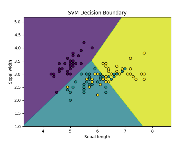
7. Visualize Results
Example
import numpy as np
import matplotlib.pyplot as plt
from sklearn import svm, datasets
from sklearn.model_selection import train_test_split
from sklearn.metrics import accuracy_score
# Load the Iris dataset
iris = datasets.load_iris()
X = iris.data[:, :2] # Use only the first two features
y = iris.target
# Split the dataset into training and test sets
X_train, X_test, y_train, y_test = train_test_split(X, y, test_size=0.3, random_state=42)
# Create SVM classifier
clf = svm.SVC(kernel='linear') # Use linear kernel function
# Train the model
clf.fit(X_train, y_train)
# Make predictions on the test set
y_pred = clf.predict(X_test)
# Calculate accuracy
accuracy = accuracy_score(y_test, y_pred)
print(f"Model accuracy: {accuracy:.2f}")
# Plot decision boundary
def plot_decision_boundary(X, y, model):
h = .02 # Grid step size
x_min, x_max = X[:, 0].min() - 1, X[:, 0].max() + 1
y_min, y_max = X[:, 1].min() - 1, X[:, 1].max() + 1
xx, yy = np.meshgrid(np.arange(x_min, x_max, h),
np.arange(y_min, y_max, h))
Z = model.predict(np.c_[xx.ravel(), yy.ravel()])
Z = Z.reshape(xx.shape)
plt.contourf(xx, yy, Z, alpha=0.8)
plt.scatter(X[:, 0], X[:, 1], c=y, edgecolors='k', marker='o')
plt.xlabel('Sepal length')
plt.ylabel('Sepal width')
plt.title('SVM Decision Boundary')
plt.show()
plot_decision_boundary(X_train, y_train, clf)
import matplotlib.pyplot as plt
from sklearn import svm, datasets
from sklearn.model_selection import train_test_split
from sklearn.metrics import accuracy_score
# Load the Iris dataset
iris = datasets.load_iris()
X = iris.data[:, :2] # Use only the first two features
y = iris.target
# Split the dataset into training and test sets
X_train, X_test, y_train, y_test = train_test_split(X, y, test_size=0.3, random_state=42)
# Create SVM classifier
clf = svm.SVC(kernel='linear') # Use linear kernel function
# Train the model
clf.fit(X_train, y_train)
# Make predictions on the test set
y_pred = clf.predict(X_test)
# Calculate accuracy
accuracy = accuracy_score(y_test, y_pred)
print(f"Model accuracy: {accuracy:.2f}")
# Plot decision boundary
def plot_decision_boundary(X, y, model):
h = .02 # Grid step size
x_min, x_max = X[:, 0].min() - 1, X[:, 0].max() + 1
y_min, y_max = X[:, 1].min() - 1, X[:, 1].max() + 1
xx, yy = np.meshgrid(np.arange(x_min, x_max, h),
np.arange(y_min, y_max, h))
Z = model.predict(np.c_[xx.ravel(), yy.ravel()])
Z = Z.reshape(xx.shape)
plt.contourf(xx, yy, Z, alpha=0.8)
plt.scatter(X[:, 0], X[:, 1], c=y, edgecolors='k', marker='o')
plt.xlabel('Sepal length')
plt.ylabel('Sepal width')
plt.title('SVM Decision Boundary')
plt.show()
plot_decision_boundary(X_train, y_train, clf)
Execute the above code, the output is:
模型准确率: 0.80
The image displays as: