Ensemble Methods
In machine learning, you may have already learned how to train a decision tree or a logistic regression model. The performance of a single model (which we call a base learner) can sometimes hit a bottleneck.
At this point, a powerful idea emerges:Ensemble methods, which do not rely on creating a brand-new, more complex algorithm, but instead build a more powerful, more stable, and more accurate super-model by cleverly combining multiple relatively simple, even mediocre models.
In simple terms, the core philosophy of ensemble learning isThree cobblers with their wits combined can outdo Zhuge Liang.。
Ensemble methods aggregate the collective wisdom of multiple models to compensate for the bias, variance, or random errors that a single model may have, thereby significantly improving overall prediction performance.
This article will systematically explain the principles, mainstream techniques, and engineering practices of ensemble methods.
Basic Ideas and Advantages of Ensemble Learning
Before diving into specific methods, we first need to understand why ensemble learning works and what benefits it can bring.
Core Idea: Reducing Error
The prediction error of a model can usually be decomposed into three parts:Bias、VarianceandIrreducible error。
- Bias: Systematic error caused by incorrect assumptions about the nature of the problem. High bias means the modelunderfitsand cannot capture the basic relationships in the data.
- Variance: The sensitivity of the model to small fluctuations in the training data. High variance means the modeloverfitsand pays too much attention to the noise in the training data.
- Irreducible error: The inherent random noise in the data, which cannot be eliminated by any model.
The core goal of ensemble methods is to combine multiple models toreduce the variance or bias of the overall model, thereby obtaining more robust (stable) and more accurate predictions.
Main Advantages
- Improve accuracy: This is the most direct goal; ensemble models outperform the best single base learner in the vast majority of scenarios.
- Enhance stability and robustness: Through averaging or voting, ensemble models are less sensitive to noisy data and outliers, reducing the risk of overfitting.
- Expand the hypothesis space: Combining multiple models is equivalent to exploring a broader solution space, making it more likely to approach the optimal solution to the problem.
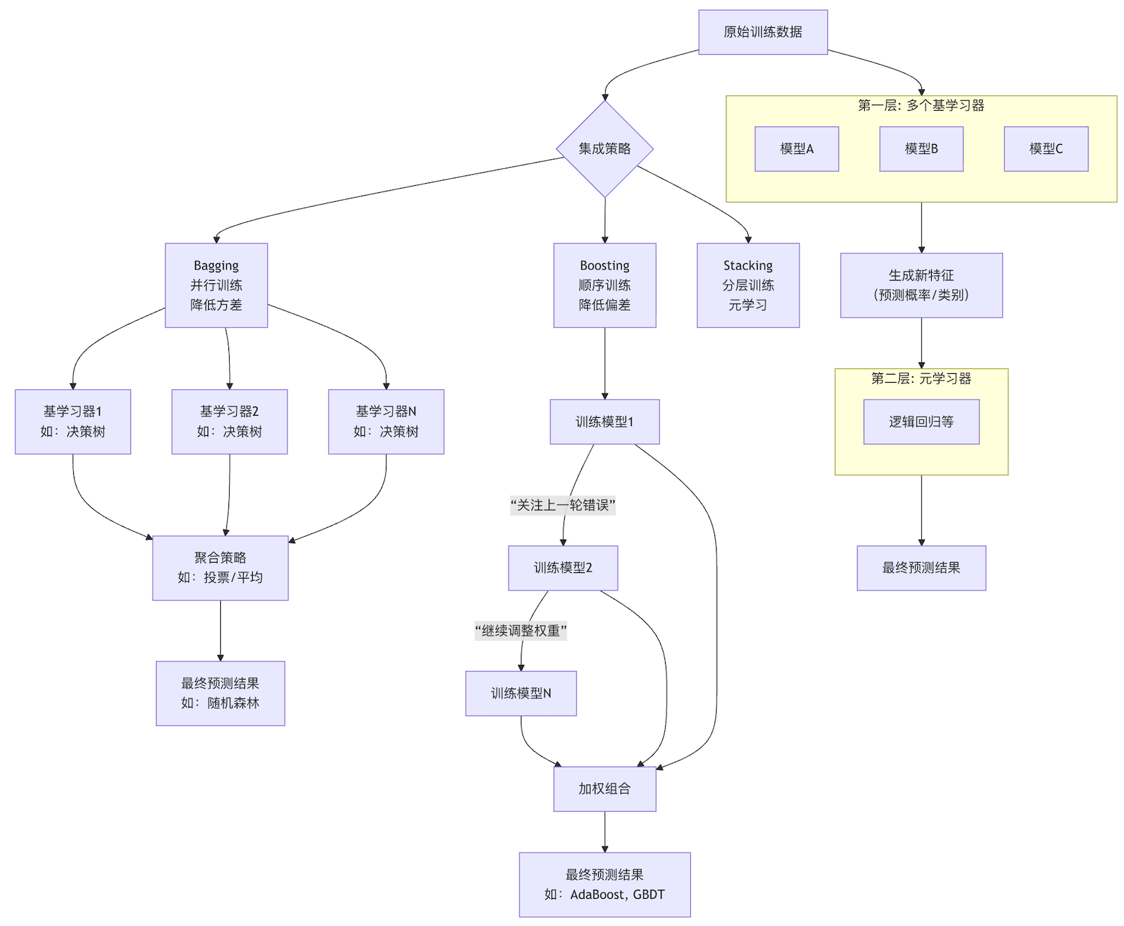
To more intuitively understand how ensemble methods work by combining multiple models, we can look at the following flowchart:
Detailed Explanation of Mainstream Ensemble Methods
According to the generation method and combination strategy of base learners, ensemble methods are mainly divided into three categories:Bagging、BoostingandStacking。
Bagging: The Path of Parallelism, Stability First
BaggingThe core idea isBootstrap Aggregating。
- Bootstrap: From the original training set, performsampling with replacementrandom sampling to generate multiple different training subsets. The size of each subset may be the same as the original set, but because of sampling with replacement, some samples will be drawn repeatedly while others will not be drawn at all.
- Parallel training: Use the same learning algorithm (usually a high-variance, low-bias model, such as an unpruned decision tree) to independently train a base learner on each subset.
- Aggregating: For classification tasks, usevoting(majority rule) to determine the final class; for regression tasks, useaveragingto calculate the final value.
Representative Algorithm: Random ForestRandom Forest is an outstanding representative of the Bagging idea. It goes one step further based on Bagging: when each decision tree performs node splitting, it not only randomly samples samples, but alsorandomly selects a subset of featuresto perform the optimal split. This "double randomness" further enhances the model's diversity and anti-overfitting ability.
Example
from sklearn.ensemble import RandomForestClassifier
from sklearn.datasets import load_iris
from sklearn.model_selection import train_test_split
from sklearn.metrics import accuracy_score
# Load data
iris = load_iris()
X, y = iris.data, iris.target
# Split training and test sets
X_train, X_test, y_train, y_test = train_test_split(X, y, test_size=0.3, random_state=42)
# Create random forest classifier
# n_estimators: number of trees in the forest, number of base learners
# max_depth: maximum depth of the tree, controls model complexity
# random_state: random seed, ensures reproducible results
rf_clf = RandomForestClassifier(n_estimators=100, max_depth=5, random_state=42)
# Train the model
rf_clf.fit(X_train, y_train)
# Predict and evaluate
y_pred = rf_clf.predict(X_test)
print(f"Random Forest Accuracy: {accuracy_score(y_test, y_pred):.4f}")
# View the depth of a single tree (example)
print(f"First tree depth: {rf_clf.estimators_)
Boosting: The Wisdom of Sequential Training, Focus on Error Correction
BoostingIt adopts a completely different strategy.
- Sequential training: The base learners aretrained sequentially, rather than in parallel.
- Focus on errors: Each subsequent model pays more attention to the samples that previous modelspredicted incorrectly.This is usually achieved by adjusting the weights of training samples (giving higher weights to misclassified samples).
- Weighted combination: Combine all base learners withweighted summationto obtain the final model; base learners that perform well have higher weights.
The core of Boosting is to continuously correct the mistakes of predecessors, elevating a group of "weak learners" (only slightly better than random guessing) into a powerful "strong learner".
Representative Algorithms: AdaBoost and Gradient Boosting Decision Tree
- AdaBoost: One of the earliest Boosting algorithms. It increases the weights of misclassified samples, forcing subsequent models to focus on these "hard" samples.
- Gradient Boosting Decision Tree (GBDT): One of the most popular and powerful Boosting algorithms. It no longer adjusts sample weights, but instead treats the training process as agradient descentoptimization process. The goal of each new tree is to fit theresiduals(negative gradient) between the current model's predictions and the true labels.
Example
from sklearn.ensemble import GradientBoostingClassifier
# Create gradient boosting classifier
# n_estimators: number of boosting stages (number of trees)
# learning_rate: learning rate, controls the contribution of each tree to the final result (shrinkage coefficient)
# max_depth: maximum depth of each regression tree, usually small (3-5), representing weak learners
gb_clf = GradientBoostingClassifier(n_estimators=100, learning_rate=0.1, max_depth=3, random_state=42)
# Train the model
gb_clf.fit(X_train, y_train)
# Predict and evaluate
y_pred_gb = gb_clf.predict(X_test)
print(f"Gradient Boosting Tree Accuracy: {accuracy_score(y_test, y_pred_gb):.4f}")
# View feature importance (ensemble methods usually provide this)
print("Feature Importance:", gb_clf.feature_importances_)
Output:
随机森林准确率: 1.0000
第一棵树的深度: 4
Stacking: Model Stacking, Meta-Learning Strategy
StackingIt is a more advanced ensemble technique that introduces the concept of a "meta-learner".
- First layer: Diverse base learners. Usedifferentlearning algorithms (such as KNN, SVM, decision trees) to train multiple models on the original data.
- Generate new features: Use these first-layer models to predict the training data (usually using cross-validation to avoid data leakage), and use their prediction results (class labels or probabilities) asnew features。
- Second layer: Train the meta-learner. With these new features as input and the original labels as output, train a final model (such as logistic regression or linear regression). This meta-learner is responsible for learning how to best combine the outputs of the first-layer models.
Stacking has great potential, but it is computationally expensive and needs careful design to prevent overfitting.
Method Comparison and Engineering Practice Recommendations
After understanding the principles, how do you choose and apply these methods in real-world projects?
Comparison of the Three Methods
| Feature | Bagging (e.g., Random Forest) | Boosting (e.g., GBDT, XGBoost) | Stacking |
|---|---|---|---|
| Core Objective | Reduce variance, prevent overfitting | Reduce bias, improve predictive power | Optimize combination strategy |
| Training method | Parallel, independent training | Sequential, depends on previous round results | Layered, base learners first then meta-learner |
| Sample weights | Treated equally, bootstrap sampling | Dynamically adjusted, focus on errors | Usually equal |
| Base learner relationship | Mutually independent, diversity comes from data perturbation | Mutually dependent, jointly optimize the objective | Mutually independent, diversity comes from algorithm differences |
| Advantages | Stable, resistant to overfitting, easy to parallelize | Prediction accuracy is usually very high | Theoretically can achieve best performance |
| Disadvantages | Limited bias reduction, high computational resource consumption | Sensitive to noise, prone to overfitting, complex tuning | Extremely high computational cost, complex structure, prone to overfitting |
| Typical applications | Random Forest, Extra-Trees | AdaBoost, GBDT, XGBoost, LightGBM, CatBoost | Common in machine learning competitions |
Engineering Practice Guide
Preferred baseline model: Don't use complex ensemble methods from the start. First use a simple model (such as logistic regression, a single decision tree) to establish a performance baseline.
Choose according to the problem:
- If your base model (such as a very deep decision tree)overfits severely (high variance), prioritize tryingBagging(Random Forest).
- If your base modelunderfits (high bias), or you pursue extremely high prediction accuracy, prioritize tryingBoosting(such as XGBoost, LightGBM).
- InMachine learning competitionsor scenarios with extreme precision requirements, and sufficient computing resources, you can considerStackingorBlending。
Use modern optimized libraries: In practice, directly use highly optimized libraries that implement state-of-the-art ensemble algorithms:
- Scikit-learn: provides
RandomForest,GradientBoostingand other excellent implementations, suitable for beginners and rapid prototyping. - XGBoost: Fast, high accuracy, full-featured, a frequent winner in Kaggle competitions.
- LightGBM: Launched by Microsoft, faster training speed, less memory consumption, especially suitable for large datasets.
- CatBoost: Launched by Yandex, handles categorical features well, and performs well with default parameters.
Pay attention to tuning: Ensemble models have many hyperparameters. Key parameters to focus on include:
n_estimators: Number of base learners (the more the better, but computational cost increases).learning_rate(Boosting): Learning rate, controls the contribution of each step. Usually needs to ben_estimatorstraded off (small learning rate requires more trees).max_depth(Tree method): Key to controlling model complexity and overfitting.- Usecross-validationandgrid search/random searchto systematically tune parameters.