Machine Learning Algorithms
Machine learning algorithms can be divided into categories such as supervised learning, unsupervised learning, and reinforcement learning.
Supervised Learning Algorithms:
- Linear Regression(Linear Regression): Used for regression tasks, predicting continuous values.
- Logistic Regression(Logistic Regression): Used for binary classification tasks, predicting categories.
- Support Vector Machine(SVM): Used for classification tasks, constructing a hyperplane for classification.
- Decision Tree(Decision Tree): A classification or regression method that makes decisions based on a tree structure.
Unsupervised Learning Algorithms:
- K-means Clustering: Groups data by cluster centers.
- Principal Component Analysis (PCA): Used for dimensionality reduction, extracting the principal components of data.
Each algorithm has its applicable scenarios. In practical applications, you can choose the most appropriate machine learning algorithm based on the characteristics of the data (such as whether there are labels, data dimensions, etc.).
| Classification Dimension | Category | Core Definition | Typical Algorithms | Core Advantages and Disadvantages | Applicable Scenarios |
|---|---|---|---|---|---|
| Learning Method | Supervised Learning | Learn the mapping from inputs to outputs using labeled data | Logistic Regression, SVM, Decision Tree, CNN, LSTM | Advantages: high prediction accuracy; Disadvantages: relies on high-quality labeled data | Classification, regression, image recognition, text translation |
| Unsupervised Learning | Use unlabeled data to mine intrinsic patterns in data | K-Means, PCA, DBSCAN, Autoencoders | Advantages: no labeling required; Disadvantages: weak interpretability of results | Data clustering, dimensionality reduction, anomaly detection, user segmentation | |
| Semi-supervised Learning | Train with a small amount of labeled data and a large amount of unlabeled data | Semi-supervised SVM, label propagation algorithms | Advantages: reduces labeling cost; Disadvantages: complex model design | Medical imaging analysis, NLP for niche languages | |
| Reinforcement Learning | The model optimizes its policy through interaction with the environment and reward signals | Q-Learning、DQN、PPO | Advantages: suitable for dynamic decision-making; Disadvantages: long training cycles | Game AI, robot control, recommendation policy optimization | |
| Task Objective | Classification Algorithms | Predict discrete class labels | Logistic Regression, Random Forest, CNN | Advantages: suitable for classification scenarios; Disadvantages: sensitive to class imbalance | Spam detection, image classification, disease diagnosis |
| Regression Algorithms | Predict continuous numerical outputs | Linear Regression, Ridge Regression, XGBoost | Advantages: outputs continuous values; Disadvantages: sensitive to outliers | Housing price prediction, sales prediction, temperature prediction | |
| Clustering Algorithms | Group similar data into one class without labels | K-Means, Hierarchical Clustering, DBSCAN | Advantages: automatic grouping; Disadvantages: clustering effect depends on distance metric | Market segmentation, user profiling, anomaly detection | |
| Dimensionality Reduction Algorithms | Reduce feature dimensions while retaining core information | PCA、t-SNE、LDA | Advantages: reduces computational cost; Disadvantages: may lose some information | High-dimensional data visualization, feature preprocessing | |
| Model Structure | Linear Models | Assume a linear relationship between input and output | Linear Regression, Logistic Regression, Ridge Regression | Advantages: strong interpretability, fast training; Disadvantages: difficult to fit nonlinear relationships | Simple classification/regression, baseline model building |
| Tree Models | Built on decision trees, handle nonlinear relationships | Decision Tree, Random Forest, XGBoost, LightGBM | Advantages: no feature normalization needed; Disadvantages: overly deep trees are prone to overfitting | Industrial-grade classification/regression, competition-level tasks | |
| Neural Network Models | Multi-layer neuron structures that automatically extract complex features | ANN、CNN、RNN、Transformer | Advantages: fits complex relationships; Disadvantages: requires large amounts of data and computing power | Image recognition, NLP, speech synthesis | |
| Probabilistic Models | Based on probability and statistics theory, compute probability distributions | Naive Bayes, Hidden Markov Models | Advantages: solid theoretical foundation; Disadvantages: relies on strong assumptions | Text classification, speech recognition, sequence labeling |
Supervised Learning Algorithms
Linear Regression
Linear regression is an algorithm for regression problems. It predicts a continuous output by learning the linear relationship between input features and target values.
Application scenarios:Predicting house prices, stock prices, etc.
The goal of linear regression is to find an optimal linear equation:

- y is the predicted value (target value).
- x1,x2,xnis the input feature.
- w1,w2,wnare the weights to be learned (model parameters).
- b is the bias term.
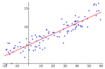
Next, we use sklearn to perform a simple housing price prediction:
Example
from sklearn.model_selection import train_test_split
import pandas as pd
# Suppose we have a simple housing price dataset
data = {
'area': [50, 60, 80, 100, 120],
'price': [150, 180, 240, 300, 350]
}
df = pd.DataFrame(data)
# Features and labels
X = df[['area']]
y = df['price']
# Data split
X_train, X_test, y_train, y_test = train_test_split(X, y, test_size=0.2, random_state=42)
# Train a linear regression model
model = LinearRegression()
model.fit(X_train, y_train)
# Predict
y_pred = model.predict(X_test)
print(f"Predicted housing price: {y_pred}")
The output is:
预测的房价: [180.8411215]
Logistic Regression
Logistic regression is an algorithm for classification problems. Despite the "regression" in its name, it is used for binary classification problems.
Logistic regression predicts a class label by learning the relationship between input features and categories.
Application scenarios:Spam classification, disease diagnosis (whether the disease is present).
The output of logistic regression is a probability value, representing the probability that a sample belongs to a certain class.
Usually uses the Sigmoid function:

Use logistic regression for a binary classification task:
Example
from sklearn.datasets import load_iris
from sklearn.model_selection import train_test_split
from sklearn.metrics import accuracy_score
# Load the Iris dataset
iris = load_iris()
X = iris.data
y = iris.target
# Take only the first two classes for binary classification
X = X[y != 2]
y = y[y != 2]
# Data split
X_train, X_test, y_train, y_test = train_test_split(X, y, test_size=0.2, random_state=42)
# Train a logistic regression model
model = LogisticRegression()
model.fit(X_train, y_train)
# Predict
y_pred = model.predict(X_test)
# Evaluate the model
print(f"Classification accuracy: {accuracy_score(y_test, y_pred):.2f}")
The output is:
分类准确率: 1.00
Support Vector Machine (SVM)
Support Vector Machine is a commonly used classification algorithm. It constructs a hyperplane to maximize the margin between classes, minimizing classification error.
Application scenarios:Text classification, face recognition, etc.
Use SVM for the Iris classification task:
Example
from sklearn.datasets import load_iris
from sklearn.model_selection import train_test_split
from sklearn.metrics import accuracy_score
# Load the Iris dataset
iris = load_iris()
X = iris.data
y = iris.target
# Data split
X_train, X_test, y_train, y_test = train_test_split(X, y, test_size=0.3, random_state=42)
# Train the SVM model
model = SVC(kernel='linear')
model.fit(X_train, y_train)
# Predict
y_pred = model.predict(X_test)
# Evaluate the model
print(f"SVM classification accuracy: {accuracy_score(y_test, y_pred):.2f}")
The output is:
SVM 分类准确率: 1.00
Decision Tree
A decision tree is a classification and regression method based on tree structures for decision-making. It determines which class a sample belongs to through a series of "judgment conditions".
Application scenarios:Customer classification, credit scoring, etc.
Use a decision tree for a classification task:
Example
from sklearn.datasets import load_iris
from sklearn.model_selection import train_test_split
from sklearn.metrics import accuracy_score
# Load the Iris dataset
iris = load_iris()
X = iris.data
y = iris.target
# Data split
X_train, X_test, y_train, y_test = train_test_split(X, y, test_size=0.3, random_state=42)
# Train a decision tree model
model = DecisionTreeClassifier(random_state=42)
model.fit(X_train, y_train)
# Prediction
y_pred = model.predict(X_test)
# Evaluate the model
print(f"Decision tree classification accuracy: {accuracy_score(y_test, y_pred):.2f}")
The output result is:
决策树分类准确率: 1.00
Unsupervised Learning Algorithms
K-means Clustering
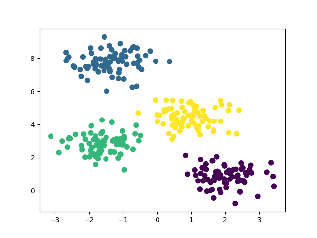
K-means is a centroid-based clustering algorithm that continuously adjusts the cluster centroids so that data points in each cluster are as close to the cluster center as possible.
Application scenarios:Customer segmentation, market analysis, image compression.
Using K-means for customer segmentation:
Example
from sklearn.datasets import make_blobs
import matplotlib.pyplot as plt
# Generate a simple 2D dataset
X, _ = make_blobs(n_samples=300, centers=4, cluster_std=0.60, random_state=0)
# Train K-means model
model = KMeans(n_clusters=4)
model.fit(X)
# Predict clustering results
y_kmeans = model.predict(X)
# Visualize clustering results
plt.scatter(X[:, 0], X[:, 1], c=y_kmeans, s=50, cmap='viridis')
plt.show()
The output figure is shown below:
Principal Component Analysis (PCA)
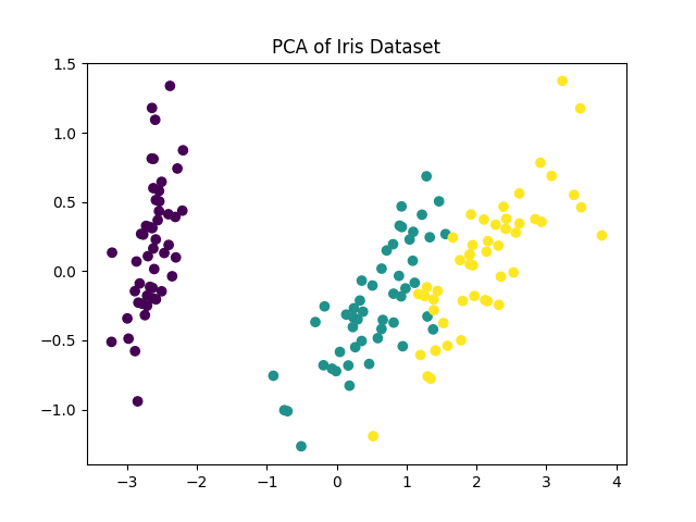
PCA is a dimensionality reduction technique that transforms data into a new coordinate system through linear transformation, concentrating most of the variance in the first few principal components.
Application scenarios:Image dimensionality reduction, feature selection, data visualization.
Using PCA for dimensionality reduction and visualizing high-dimensional data:
Example
from sklearn.datasets import load_iris
import matplotlib.pyplot as plt
# Load the Iris dataset
iris = load_iris()
X = iris.data
y = iris.target
# Reduce to 2 dimensions
pca = PCA(n_components=2)
X_pca = pca.fit_transform(X)
# Visualize the results
plt.scatter(X_pca[:, 0], X_pca[:, 1], c=y, cmap='viridis')
plt.title('PCA of Iris Dataset')
plt.show()
The output figure is shown below:
Machine Learning Algorithms
| Chinese full name | English full name | Abbreviation | Core applicable scenarios |
|---|---|---|---|
| Traditional machine learning algorithms | |||
| Decision Tree | Decision Tree | DT | Classification, regression, feature importance analysis |
| Random Forest | Random Forest | RF | Classification, regression, anomaly detection, feature selection |
| Logistic Regression | Logistic Regression | LR | Binary classification tasks, probability prediction, credit scoring |
| Support Vector Machine | Support Vector Machine | SVM | Classification, high-dimensional small-sample data, text classification |
| Naive Bayes | Naive Bayes | NB | Text classification, spam detection, sentiment analysis |
| Gradient Boosting Tree | Gradient Boosting Decision Tree | GBDT | Classification, regression, ranking tasks |
| Extreme Gradient Boosting | Extreme Gradient Boosting | XGBoost | High-precision classification and regression, competition-level tasks, click-through rate prediction |
| Light Gradient Boosting Machine | Light Gradient Boosting Machine | LightGBM | Large-scale data classification and regression, real-time prediction, recommendation systems |
| K-Nearest Neighbors Algorithm | K-Nearest Neighbor | KNN | Simple classification and regression, recommendation systems, anomaly detection |
| K-Means Clustering | K-Means Clustering | K-Means | Data clustering, user segmentation, image segmentation |
| Principal Component Analysis | Principal Component Analysis | PCA | Data dimensionality reduction, high-dimensional data visualization, feature denoising |
| Deep learning algorithms | |||
| Artificial Neural Network | Artificial Neural Network | ANN | Simple classification and regression, baseline model validation |
| Convolutional Neural Network | Convolutional Neural Network | CNN | Image recognition, object detection, video analysis, medical image diagnosis |
| Recurrent Neural Network | Recurrent Neural Network | RNN | Sequence data processing, text generation, speech recognition |
| Long Short-Term Memory Network | Long Short-Term Memory | LSTM | Long-sequence text translation, speech synthesis, time series prediction |
| Gated Recurrent Unit | Gated Recurrent Unit | GRU | Sequence classification, sentiment analysis, dialogue systems |
| Generative Adversarial Network | Generative Adversarial Network | GAN | Image generation, style transfer, data augmentation, super-resolution reconstruction |
| Transformer | Transformer | Transformer | Natural language translation, text summarization, multimodal tasks, foundation architecture for large models |
| Autoencoder | Autoencoder | AE | Data compression, anomaly detection, feature extraction |
| Variational Autoencoder | Variational Autoencoder | VAE | Generative tasks, data denoising, image generation |
| Graph Neural Network | Graph Neural Network | GNN | Social network analysis, molecular structure prediction, knowledge graph reasoning |