Classification Metrics
In the world of machine learning, building a classification model is only the first step. Just as a doctor cannot judge an illness by intuition alone, we also need a set of scientifichealth check metricsto evaluate the health of the model. These metrics areclassification metrics, which can tell us how accurate the model's predictions are, what it does well, and where it falls short.
Today, we will learn about these crucial evaluation tools together.
Why Do We Need Classification Metrics?
Imagine you trained a model to identify whether an email is spam. The model made predictions on 100 emails, and you might ask:
- "How many did it predict correctly?" -> This leads toaccuracy。
- "Of the actual spam emails, how many did it find?" -> This leads torecall。
- "Of the emails it said were spam, how many are actually spam?" -> This leads toprecision。
If we only judge by how many were correct, it is like evaluating a student only by total exam score, ignoring a lot of important information. Different business scenarios have different priorities:
- Disease diagnosis: We care more about not missing any patient (high recall), even if it means examining more healthy people (sacrificing some precision).
- Spam filtering: We care more about not throwing important emails into the junk folder (high precision), even if it means missing some spam emails (sacrificing some recall).
Therefore, we need a series of metrics to comprehensively evaluate model performance from different perspectives.
Core Concept: Confusion Matrix
Almost all classification metrics originate from a powerful tool—the confusion matrix.It is a "panoramic map" for understanding the model's prediction results.
What Is a Confusion Matrix?
It is a table that shows all four possible situations between the model's predicted results and the true labels.
Example
from sklearn.metrics import confusion_matrix
import seaborn as sns
import matplotlib.pyplot as plt
# Assume we have true labels and predicted labels
y_true = [1, 0, 1, 1, 0, 0, 1, 0, 0, 1] # 1 represents spam, 0 represents normal email
y_pred = [1, 0, 0, 1, 0, 0, 1, 1, 0, 1] # Model predictions
# Compute the confusion matrix
cm = confusion_matrix(y_true, y_pred)
print("Confusion matrix:")
print(cm)
# The output might be:
# [[4 1] # True is 0 (normal), 4 predicted as 0 (TN), 1 predicted as 1 (FP)
# [1 4]] # True is 1 (spam), 1 predicted as 0 (FN), 4 predicted as 1 (TP)
To better understand it, let's visualize it:
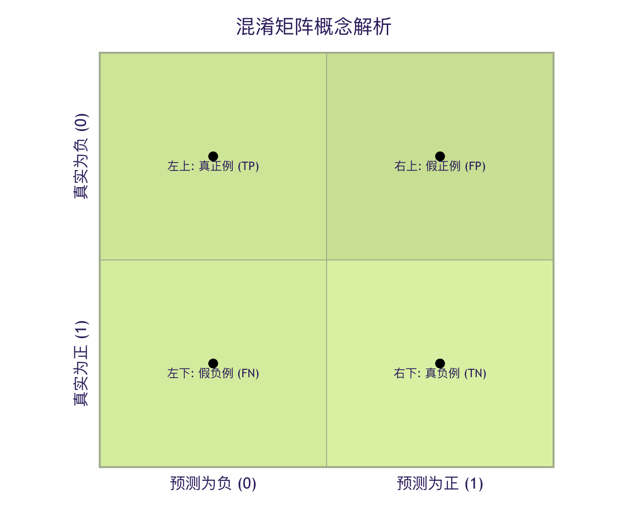
Let's break down these four core terms:
| Term | Abbreviation | Meaning | Explanation in the spam example |
|---|---|---|---|
| True Positive | TP | Model predicted ascorrect, and the actual is alsocorrect。 | Correctly identified by the modelspam emails。 |
| False Positive | FP | Model predicted ascorrect, but the actual isnegative。 | The modelmisclassifiesas spamnormal emails。 (Type I Error) |
| True Negative | TN | Model predicted asnegative, and the actual is alsonegative。 | Correctly identified by the modelnormal emails。 |
| False Negative | FN | Model predicted asnegative, but the actual iscorrect。 | The modelmissedofspam emails。 (Type II Error) |
Memory Tip:
- True/Falserefers towhether the prediction is correct。
- Positive/Negativerefers tothe model's prediction result。
3. Detailed Explanation of Core Classification Metrics
With the confusion matrix, we can derive various evaluation metrics just like calculating with formulas.
1. Accuracy - The Most Intuitive Metric
Accuracymeasures the proportion of correctly predicted samples out of the total samples.
\[ \text{Accuracy} = \frac{TP + TN}{TP + TN + FP + FN} \]
Example
accuracy = accuracy_score(y_true, y_pred)
print(f"Accuracy: {accuracy:.2f}") # Output: 0.80 (8/10)
Characteristics and Limitations:
- Advantages: Very intuitive and easy to understand.
- Disadvantages: Inimbalanced data,it can be misleading. For example, if 99% of emails are normal, a "dumb model" that predicts all emails as normal can achieve 99% accuracy as well, but it cannot catch a single spam email.
2. Precision - The "Quality over Quantity" Metric
Precisionfocuses on how many of the model's predictedpositive samplesare actually true positives. It measures the prediction results'reliabilityorand precision.。
\[ \text{Precision} = \frac{TP}{TP + FP} \]
Question: Among the emails we predicted as spam, how many are actually spam?High precision means: When the model says "this is spam," the credibility is very high.
Example
precision = precision_score(y_true, y_pred)
print(f"Precision: {precision:.2f}") # Output: 0.80 (TP=4, TP+FP=5)
3. Recall - The "Better to Cast a Wide Net" Metric
Recallfocuses on all actualpositive sampleshow many were found by the model. It measures the model'sability to discover positive samples.。
\[ \text{Recall} = \frac{TP}{TP + FN} \]
Question: Of all actual spam emails, how many did we find?High recall means: The model rarely misses actual spam emails.
Example
recall = recall_score(y_true, y_pred)
print(f"Recall: {recall:.2f}") # Output: 0.80 (TP=4, TP+FN=5)
4. F1 Score - The Harmonic Mean of Precision and Recall
Precision and recall are usually in tension (improving one often lowers the other).The F1 scoreis the harmonic mean of the two, aiming to find a balance.
\[ \text{F1 Score} = 2 \times \frac{\text{Precision} \times \text{Recall}}{\text{Precision} + \text{Recall}} \]
Characteristics of the Harmonic Mean: It tends to penalize extreme values. Only when both precision and recall are high will the F1 score be high.
Example
f1 = f1_score(y_true, y_pred)
print(f"F1 Score: {f1:.2f}") # Output: 0.80
Metrics Comparison and Selection Guide
| Metric | Formula | Focus | Example application scenarios |
|---|---|---|---|
| Accuracy | (TP+TN)/Total | Overall prediction accuracy | Scenarios where classes are balanced and the costs of FP and FN are similar. |
| Precision | TP/(TP+FP) | Predicted as positive:accuracy of the samples. | High FP cost.Such as spam filtering (fear of deleting important emails), recommendation systems (fear of recommending poor-quality products). |
| Recall | TP/(TP+FN) | Actually positiveThe proportion of samples that are found | FN cost is highSuch as disease screening (fear of missed diagnosis), fraud detection (fear of missing fraudulent transactions). |
| F1 score | 2PR/(P+R) | Balance of precision and recall | Scenarios that require comprehensive consideration without clear bias; better than accuracy when classes are imbalanced. |
4. Advanced Metrics: ROC Curve and AUC
When the model's prediction result is a probability value (e.g., the probability that an email is spam is 0.8), we need to set athreshold(e.g., 0.5) to decide the final classification. The ROC curve helps us evaluate the model's overall performance under different thresholds.
1. True Positive Rate and False Positive Rate
- True positive rate (TPR): is actuallyrecall。TPR = TP / (TP + FN)
- False positive rate (FPR): The proportion of all actual negative samples that are incorrectly predicted as positive. FPR = FP / (FP + TN)
2. ROC Curve
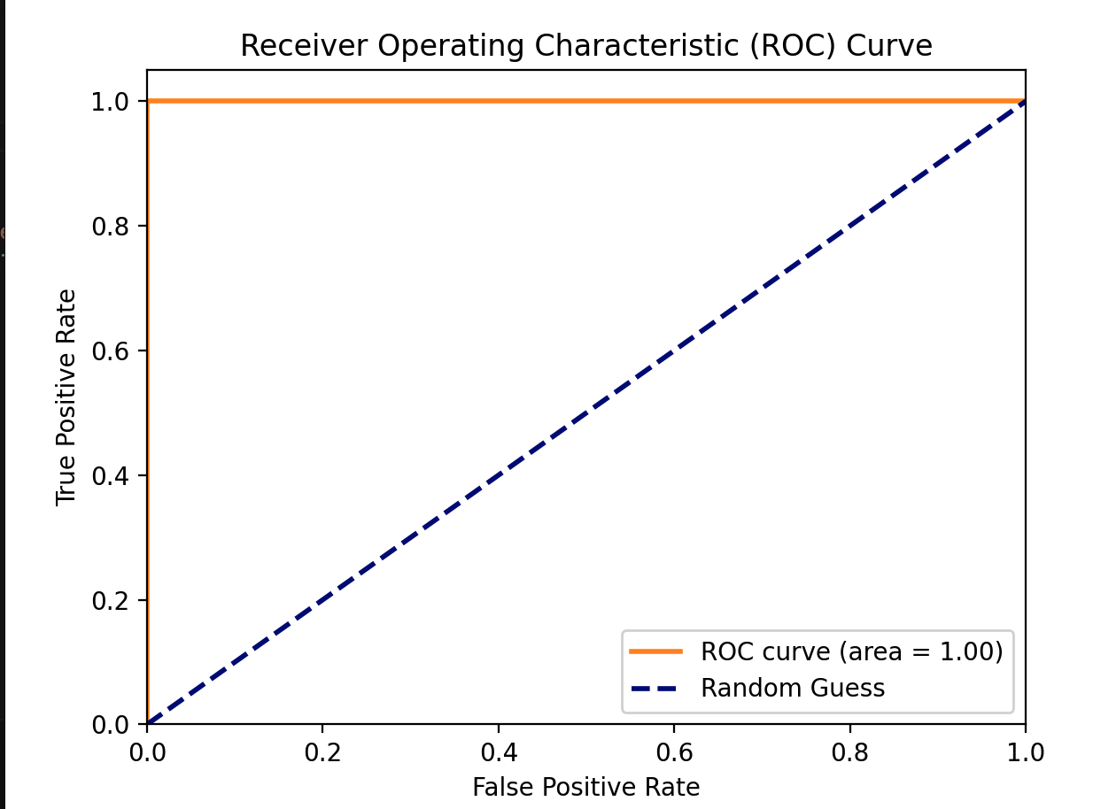
The ROC curve usesFPR as the horizontal axis,TPR as the vertical axis. Each point on the curve corresponds to a specific classification threshold.
- Ideal point: top-left corner (0, 1), i.e., FPR=0 (no false positives), TPR=1 (all recalled).
- Random line: diagonal from (0,0) to (1,1), representing the performance of a random guessing model.
3. AUC Value
AUC is the area under the ROC curve.
- AUC = 1: perfect model.
- AUC = 0.5: the model has no discriminative ability, equivalent to random guessing.
- 0.5 < AUC < 1: the model has some predictive ability, the larger the value the better.
- AUC < 0.5: the model is worse than random guessing, usually meaning the prediction direction is reversed.
The advantage of AUC is that itis insensitive to class imbalance, and it evaluates the model's overall ranking ability (the ability to rank positive samples ahead of negative samples).
Example
import numpy as np
import matplotlib.pyplot as plt
# Suppose we have some predicted probabilities (simulated here with random numbers)
y_true = [1, 0, 1, 0, 1]
y_scores = [0.9, 0.4, 0.6, 0.3, 0.8] # Probability of the model predicting a positive example
fpr, tpr, thresholds = roc_curve(y_true, y_scores)
roc_auc = auc(fpr, tpr)
print(f"AUC value: {roc_auc:.2f}")
# Plot the ROC curve (optional, requires matplotlib)
plt.figure()
plt.plot(fpr, tpr, color='darkorange', lw=2, label=f'ROC curve (area = {roc_auc:.2f})')
plt.plot([0, 1], [0, 1], color='navy', lw=2, linestyle='--', label='Random Guess')
plt.xlim([0.0, 1.0])
plt.ylim([0.0, 1.05])
plt.xlabel('False Positive Rate')
plt.ylabel('True Positive Rate')
plt.title('Receiver Operating Characteristic (ROC) Curve')
plt.legend(loc="lower right")
plt.show()
Output:
AUC 值: 1.00
Metrics for Multi-class Classification Problems
When there are more than two classes (e.g., identifying cats, dogs, rabbits), the above metrics can be extended in the following ways:
- Macro average: First compute the metric for each class (e.g., precision), then take the arithmetic mean of the metrics for all classes.Treat each class equally。
- Micro average: First aggregate the TP, FP, etc. of all classes, then use the aggregated values to compute a global metric.Treat each sample equally, more influenced by large classes.
In Scikit-learn, you can specify viaaveragethe parameters:
Example
# y_true and y_pred are now multi-class labels, e.g., [0, 1, 2, 0, 1]
precision_macro = precision_score(y_true, y_pred, average='macro') # Macro average
precision_micro = precision_score(y_true, y_pred, average='micro') # Micro average
6. Practical Exercise: Comprehensive Evaluation of a Classification Model
Now, let's practice with a real dataset. We will use the famous Iris dataset.
Example
from sklearn.model_selection import train_test_split
from sklearn.linear_model import LogisticRegression
from sklearn.metrics import classification_report, confusion_matrix, accuracy_score
# 1. Load data
iris = load_iris()
X = iris.data
y = iris.target
target_names = iris.target_names
# 2. Split into training and test sets
X_train, X_test, y_train, y_test = train_test_split(X, y, test_size=0.3, random_state=42)
# 3. Train a simple logistic regression model
model = LogisticRegression(max_iter=200)
model.fit(X_train, y_train)
# 4. Make predictions on the test set
y_pred = model.predict(X_test)
y_pred_proba = model.predict_proba(X_test) # Get predicted probabilities for AUC
# 5. Compute and print various metrics
print("=== Confusion Matrix ===")
print(confusion_matrix(y_test, y_test))
# Note: the confusion matrix for multi-class is N x N
print("\n=== Classification Report (including precision, recall, F1) ===")
print(classification_report(y_test, y_pred, target_names=target_names))
# classification_report is a very convenient function that outputs multiple metrics at once.
print(f"\n=== Accuracy ===")
print(f"{accuracy_score(y_test, y_pred):.4f}")
# 6. For multi-class AUC, usually compute the "one-vs-rest" AUC for each class relative to the other classes, then take the average.
from sklearn.metrics import roc_auc_score
# Note: roc_auc_score requires specifying multi_class='ovr' (One-vs-Rest) and average for multi-class
try:
auc_ovr = roc_auc_score(y_test, y_pred_proba, multi_class='ovr', average='macro')
print(f"\n=== Macro Average AUC (OvR) ===")
print(f"{auc_ovr:.4f}")
except Exception as e:
print(f"\nError computing AUC (some classes may not appear in the test set): {e}")
Run this code and you will see a complete model evaluation report. Try modifying the model parameters or using a different model (such assklearn.tree.DecisionTreeClassifier) and observe how these metrics change.
=== 混淆矩阵 ===
[[19  0  0]
 [ 0 13  0]
 [ 0  0 13]]

=== 分类报告(包含精确率、召回率、F1)===
              precision    recall  f1-score   support

      setosa       1.00      1.00      1.00        19
  versicolor       1.00      1.00      1.00        13
   virginica       1.00      1.00      1.00        13

    accuracy                           1.00        45
   macro avg       1.00      1.00      1.00        45
weighted avg       1.00      1.00      1.00        45


=== 准确率 ===
1.0000

=== 宏平均 AUC (OvR) ===
1.0000
Other extensions