Common Network Types
Imagine we are teaching a child to recognize cats and dogs.
Initially, we show them many pictures of cats and dogs and tell them "this is a cat, this is a dog." Gradually, the child's brain extracts patterns from these images: cats usually have pointed ears and rounder faces; dogs' ears may droop and their faces are longer. This process is essentiallylearning featuresandand building patterns.。
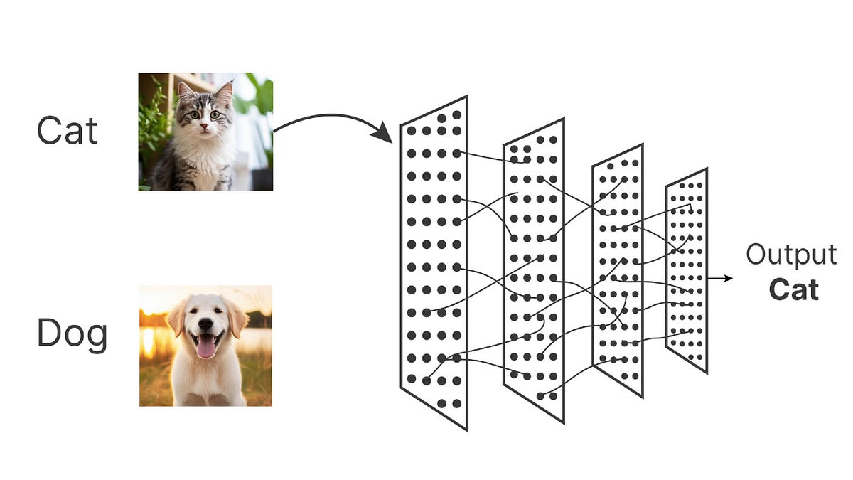
Deep learning, a powerful branch of machine learning, is centered on enabling computers to simulate this process. By building multi-layer neural networks, it allows machines to automatically learn and extract complex features from massive data, ultimately accomplishing advanced tasks such as image recognition, language understanding, and trend prediction. Different tasks require networks with different architectures. This article will introduce you to several core, common types of deep learning networks and help you understand their design philosophies and typical applications.
Deep Learning Networks
| Chinese Full Name | English Full Name | Abbreviation |
|---|---|---|
| Artificial Neural Network | Artificial Neural Network | ANN |
| Convolutional Neural Network | Convolutional Neural Network | CNN |
| Recurrent Neural Network | Recurrent Neural Network | RNN |
| Long Short-Term Memory Network | Long Short-Term Memory | LSTM |
| Gated Recurrent Unit | Gated Recurrent Unit | GRU |
| Generative Adversarial Network | Generative Adversarial Network | GAN |
| Transformer | Transformer | Transformer |
| Autoencoder | Autoencoder | AE |
| Variational Autoencoder | Variational Autoencoder | VAE |
| Deep Belief Network | Deep Belief Network | DBN |
| Graph Neural Network | Graph Neural Network | GNN |
Neural Network Basics and Fully Connected Networks
Before diving into various networks, we need to understand the most basic model —fully connected network, also known asmulti-layer perceptron (MLP)。
Core Idea: Everything Can Be Connected
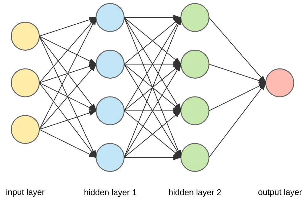
The fully connected network is the most straightforward architecture in deep learning. As the name suggests, each layer'severy neuronis connected to the adjacent layer'severy neuron.

We can think of it as an extremely dense information processing network. Data enters from the input layer, undergoes transformations through multiple hidden layers, and finally produces results at the output layer.
Typical Applications and Limitations
Application: Thanks to its powerful fitting capability, FCN is well suited for structured data (e.g., tabular data such as house area, location, and number of rooms in house price prediction).
Example
import torch.nn as nn
class SimpleFCN(nn.Module):
def __init__(self, input_size, num_classes):
super(SimpleFCN, self).__init__()
# Define network layers
self.fc1 = nn.Linear(input_size, 128) # First hidden layer
self.relu = nn.ReLU() # Activation function
self.fc2 = nn.Linear(128, 64) # Second hidden layer
self.fc3 = nn.Linear(64, num_classes) # Output layer
def forward(self, x):
x = self.fc1(x)
x = self.relu(x)
x = self.fc2(x)
x = self.relu(x)
x = self.fc3(x)
return x
# Assume input is a 100-dimensional feature, for 10-class classification
model = SimpleFCN(input_size=100, num_classes=10)
Limitations: When dealing with grid-like data such as images and speech, FCN faces significant challenges. Because pixels in an image are highly correlated in space, FCN ignores this spatial structure and flattens the image into a one-dimensional vector for processing, leading to an explosion in the number of parameters and difficulty in learning effective spatial features.
Convolutional Neural Networks — The Cornerstone of Computer Vision
To solve the problem of image processing,Convolutional Neural Networks (CNN)emerged as the times require, completely transforming the field of computer vision.
Core Idea: Local Perception and Parameter Sharing
CNN draws design inspiration from the biological visual cortex, and its two core ideas are:
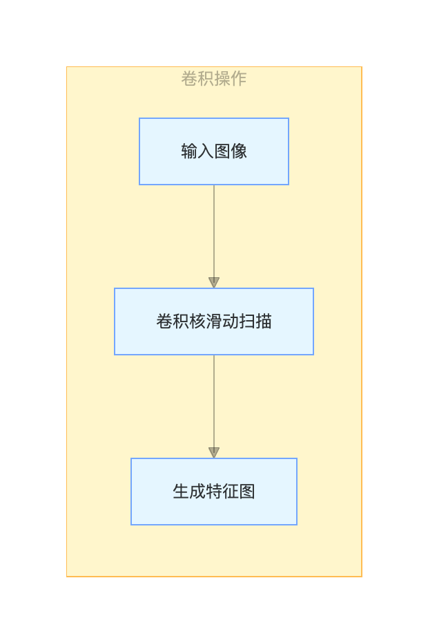
- Local perception: Unlike FCN, where neurons connect to the entire image, each neuron in CNN only perceives asmall local region(e.g., a 3x3 or 5x5 pixel patch). This better matches the property that adjacent pixels in an image are more strongly correlated.
- Parameter sharing: Using the sameconvolution kernel(or filter) to slide and scan at different positions of the image, extracting the same type of features (such as edges, textures). This greatly reduces network parameters.
Core Components and Typical Applications
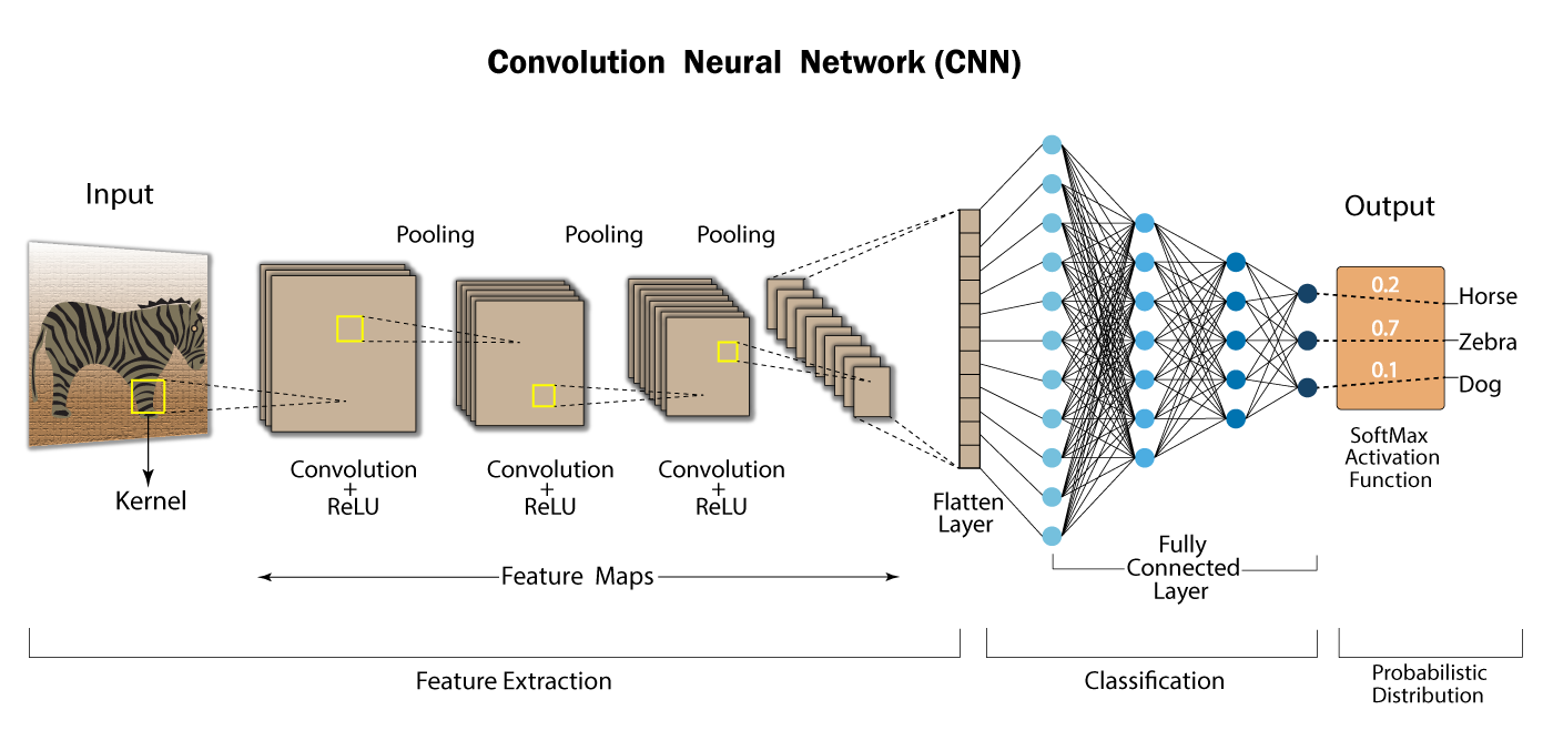
A typical CNN is stacked from the following components:
- Convolutional layer: Uses convolution kernels to extract features.
- Pooling layer(e.g., max pooling): Downsamples feature maps, reducing data volume and enhancing feature invariance.
- Fully connected layer: At the end of the network, maps learned distributed features to the sample label space.
Application: Almost all computer vision tasks such as image classification, object detection, and face recognition.
Example
class SimpleCNN(nn.Module):
def __init__(self, num_classes=10):
super(SimpleCNN, self).__init__()
self.conv1 = nn.Conv2d(in_channels=3, out_channels=16, kernel_size=3, padding=1)
self.pool = nn.MaxPool2d(kernel_size=2, stride=2)
self.conv2 = nn.Conv2d(16, 32, 3, padding=1)
self.fc1 = nn.Linear(32 * 8 * 8, 256) # Assume the feature map size is 8x8 after two pooling operations
self.fc2 = nn.Linear(256, num_classes)
def forward(self, x):
x = self.pool(nn.functional.relu(self.conv1(x))) # Convolution -> Activation -> Pooling
x = self.pool(nn.functional.relu(self.conv2(x)))
x = x.view(-1, 32 * 8 * 8) # Flatten the feature map into a one-dimensional vector
x = nn.functional.relu(self.fc1(x))
x = self.fc2(x)
return x
Recurrent Neural Networks — Experts at Processing Sequential Data
For data such as language, speech, and time series that havesequential dependency relationships, we need a network that can remember historical information. This is theRecurrent Neural Network (RNN)。
Core Idea: Introducing a Memory Mechanism
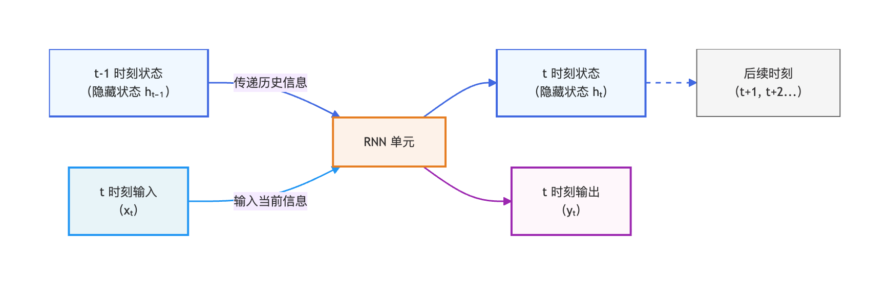
The core of RNN lies in its recurrent structure. When processing the current input, the network combines the current input with thehidden state from the previous time stepto jointly determine the current output and the hidden state passed to the next time step. This is like reading a sentence: understanding the current word requires relying on previously read words.
Variants and Typical Applications
Basic RNN suffers from the long-term dependency problem, making it difficult to learn information in long sequences. This led to two important variants:
- Long Short-Term Memory network (LSTM): Through an elaborate gating mechanism (input gate, forget gate, output gate), it selectively remembers important information and forgets useless information, effectively solving the long-sequence dependency problem.
- Gated Recurrent Unit (GRU): A simplified version of LSTM with a more concise structure and higher computational efficiency, performing comparably on many tasks.
Application: Machine translation, text generation, speech recognition, stock price prediction.
Example
class SimpleRNN(nn.Module):
def __init__(self, vocab_size, embed_size, hidden_size, num_classes):
super(SimpleRNN, self).__init__()
self.embedding = nn.Embedding(vocab_size, embed_size) # Word embedding layer
self.rnn = nn.RNN(input_size=embed_size, hidden_size=hidden_size, batch_first=True)
self.fc = nn.Linear(hidden_size, num_classes)
def forward(self, x):
# Shape of x: (batch_size, sequence_length)
x = self.embedding(x) # After embedding: (batch_size, seq_len, embed_size)
_, h_n = self.rnn(x) # h_n is the hidden state of the last time step
out = self.fc(h_n.squeeze(0)) # Use the final state for classification
return out
Generative Adversarial Networks — From Learning to Creation
If the previous networks are discriminative models (learning to distinguish data), thenGenerative Adversarial Network (GAN)is an outstanding representative of generative models (learning to create data).

Core Idea: Evolution Through Adversarial Games
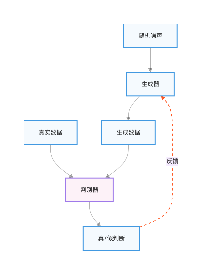
GAN draws inspiration from game theory. It consists of two adversarial networks:
- Generator: Like a forger, its goal is to learn the distribution of real data and generate new data realistic enough to pass as genuine.
- Discriminator: Like an authentication expert, its goal is to accurately distinguish whether input data comes from the real dataset or the generator.
The two improve together through continuous adversarial training: the generator strives to create more realistic data to fool the discriminator, while the discriminator works to improve its ability to distinguish. Eventually, the generator can produce high-quality new data.
Typical Applications
Application: Image generation, image super-resolution, style transfer, data augmentation.
Example
for epoch in range(num_epochs):
# 1. Train the discriminator: maximize its ability to classify real data as real and generated data as fake
real_data = get_real_data()
noise = generate_random_noise()
fake_data = generator(noise).detach() # Note the detach to prevent the generator from being updated
d_loss_real = criterion(discriminator(real_data), real_labels)
d_loss_fake = criterion(discriminator(fake_data), fake_labels)
d_loss = d_loss_real + d_loss_fake
d_loss.backward()
optimizer_D.step()
# 2. Train the generator: minimize the discriminator's ability to classify generated data as fake (i.e., fool the discriminator)
noise = generate_random_noise()
fake_data = generator(noise)
g_loss = criterion(discriminator(fake_data), real_labels) # Make the discriminator believe the generated data is real
g_loss.backward()
optimizer_G.step()
Summary and Comparison
| Network Type | Core Idea | Data Types It Excels At Processing | Typical Applications |
|---|---|---|---|
| Fully Connected Network | Global connection, dense fitting | Structured data (tables) | House price prediction, credit scoring |
| Convolutional Neural Network | Local perception, parameter sharing | Grid data (images) | Image classification, object detection |
| Recurrent Neural Network | Temporal dependency, memory state | Sequence data (text, time series) | Machine translation, speech recognition |
| Generative Adversarial Network | Adversarial game, data generation | Used to generate data similar to real data | Image generation, style transfer |