Polynomial Regression
Imagine you are observing the trajectory of an object falling from the sky. Its falling speed is not uniform, but gets faster and faster. If you use a straight line to fit this trajectory, the result will be very poor, because a straight line cannot describe this curved change. At this point, we need a line that can bend—polynomial regression is a powerful tool for solving such problems.
In simple terms,polynomial regressionis an extension of linear regression. It maps data to a higher-dimensional space by adding higher-degree terms (such as squared terms, cubic terms) to the original features, thereby using a "curve" to fit the nonlinear relationships present in the data.
1. Core Concepts: From Straight Lines to Curves
1.1 Reviewing Linear Regression
The model formula for linear regression is very simple:y = w₁ * x + bwhere:
yis the target value we want to predict.xis the input feature.w₁is the weight (slope) of the feature.bis the bias term (intercept).
This model determines that it can only draw astraight line。
1.2 Introducing Polynomial Regression
The core idea of polynomial regression is:Treat higher powers of the feature as new featuresand then apply linear regression on this expanded feature set.
For example, a quadratic polynomial regression model:y = w₁ * x + w₂ * x² + b
You see, although the equation now containsx²but if wexandx²regard them as two independent featuresX1andX2then the model becomes:y = w₁ * X1 + w₂ * X2 + bThis is essentially still alinear modelbut it is linear with respect to thefeatures X1andX2linear. This is why polynomial regression is called an "extension of linear regression".
1.3 Key Terms
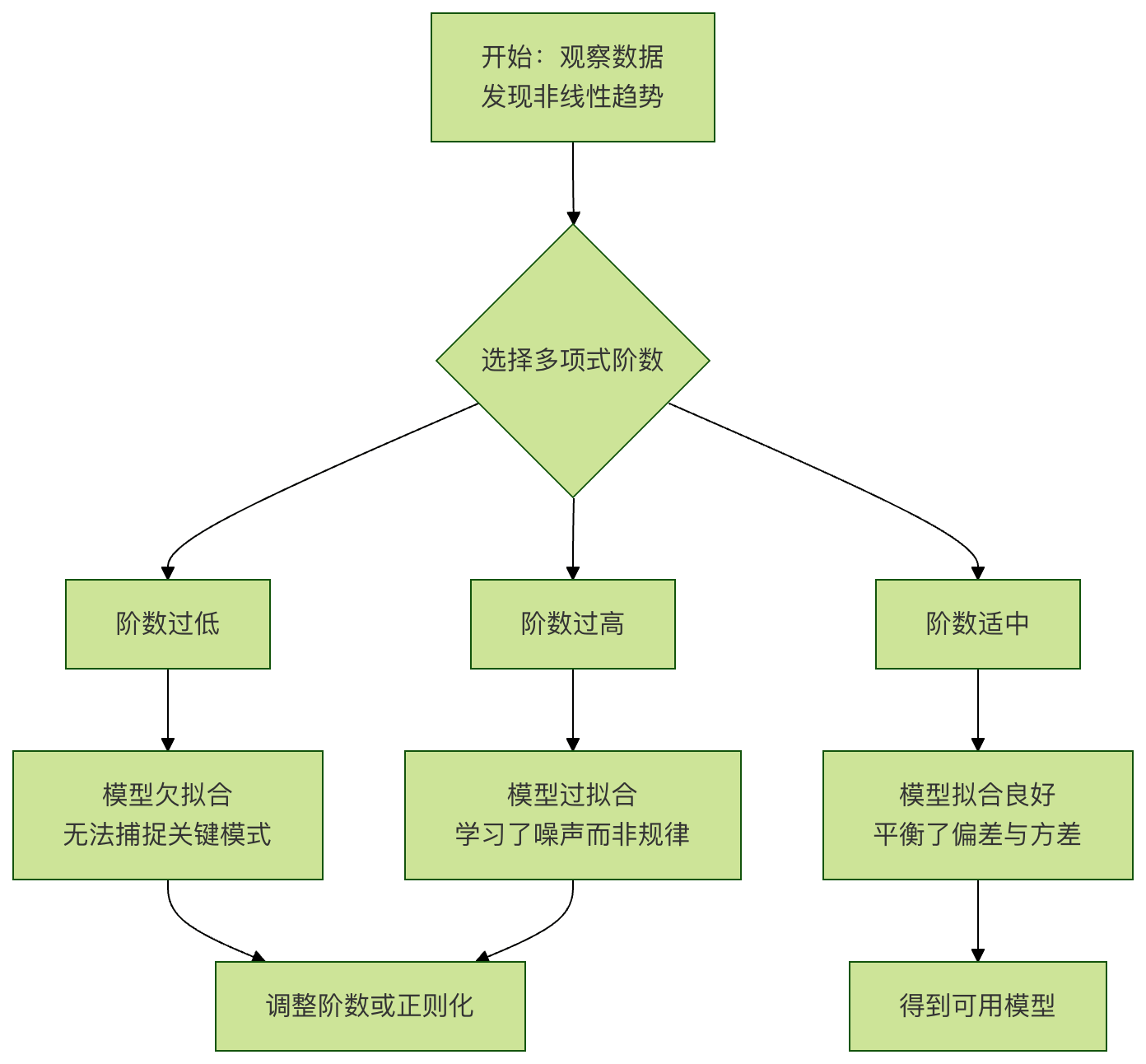
- Degree/Order: The highest exponent in the polynomial. Degree 2 is a quadratic curve (parabola), degree 3 is a cubic curve, and so on.
- Overfitting: If the chosen degree is too high, the model becomes very "twisty", perfectly passing through all training data points, but its ability to predict new data drops sharply. It's like using a complex net to catch a few points; if the mesh is too fine, it may fail to catch big fish.
- Underfitting: If the degree is too low (for example, using a straight line to fit clearly curved data), the model cannot capture the underlying pattern in the data, and its predictive ability is also poor.
The flowchart below illustrates a typical thought process for applying polynomial regression:
2. Hands-on: Implementing Polynomial Regression in Python
We will usescikit-learnthis powerful machine learning library, which makes implementing polynomial regression very simple.
2.1 Preparing the Environment and Data
First, ensure the necessary libraries are installed, and create a set of simulated nonlinear data.
Example
import numpy as np
import matplotlib.pyplot as plt
from sklearn.preprocessing import PolynomialFeatures
from sklearn.linear_model import LinearRegression
from sklearn.metrics import mean_squared_error, r2_score
# Set random seed to ensure consistent results across runs
np.random.seed(42)
# Create simulated data: y is a quadratic function of x plus some random noise
X = 6 * np.random.rand(100, 1) - 3 # Generate 100 random numbers in the interval [-3, 3)
y = 0.5 * X**2 + X + 2 + np.random.randn(100, 1) # y = 0.5x^2 + x + 2 + noise
# Visualize the original data
plt.scatter(X, y, s=10, alpha=0.7, label='Original data')
plt.xlabel('X')
plt.ylabel('y')
plt.title('Simulated nonlinear data')
plt.legend()
plt.show()
Running this code, you will see that the data points roughly follow a "U" shape (parabola) distribution, and fitting a straight line is clearly inappropriate.
2.2 Core Steps: Feature Transformation and Model Training
The key step is to usePolynomialFeaturesto generate higher-degree feature terms.
Example
# The parameter degree determines the degree of the polynomial; here we try degree 2
poly_features = PolynomialFeatures(degree=2, include_bias=False)
# Transform the original feature X into a new feature matrix X_poly containing X and X^2
X_poly = poly_features.fit_transform(X)
print(f"Original X shape: {X.shape}")
print(f"Transformed X_poly shape: {X_poly.shape}")
print(f"First 5 rows of X_poly data:\n{X_poly[:5]}")
# The output shows that X_poly has two columns: the first column is X, and the second is X^2
# 2. Train a linear regression model on the transformed features
lin_reg = LinearRegression()
lin_reg.fit(X_poly, y) # Use X_poly instead of the original X
# 3. View the learned model parameters (weights and bias)
print(f"\nModel parameters (weights w1, w2): {lin_reg.coef_.ravel()})
print(f"Model bias (intercept b): {lin_reg.intercept_}")
# The output should be close to the parameters [1, 0.5] and 2 used when generating the data
2.3 Visualizing the Fitting Results
Let's see what the trained "curve" model looks like.
Example
X_new = np.linspace(-3, 3, 100).reshape(100, 1)
# Apply the same polynomial feature transformation to these new points
X_new_poly = poly_features.transform(X_new)
# Use the model to make predictions
y_new = lin_reg.predict(X_new_poly)
# Start plotting
plt.scatter(X, y, s=10, alpha=0.7, label='Training data')
plt.plot(X_new, y_new, 'r-', linewidth=2, label='Polynomial regression fit (degree=2)')
plt.xlabel('X')
plt.ylabel('y')
plt.title('Quadratic polynomial regression fitting effect')
plt.legend()
plt.show()
You should see a nice red curve that captures the parabolic trend of the data well.
3. Important Topic: How to Choose the Correct Degree?
Choosing the degree is a trade-off process. We can intuitively understand this by visualizing the fitting effects of different degrees.
Example
degrees = [1, 2, 15]
plt.figure(figsize=(15, 4))
for i, degree in enumerate(degrees):
# Create subplots
ax = plt.subplot(1, len(degrees), i + 1)
# Generate polynomial features and train the model
poly_features = PolynomialFeatures(degree=degree, include_bias=False)
X_poly = poly_features.fit_transform(X)
lin_reg = LinearRegression()
lin_reg.fit(X_poly, y)
# Predict and plot
y_new = lin_reg.predict(poly_features.transform(X_new))
ax.scatter(X, y, s=10, alpha=0.7)
ax.plot(X_new, y_new, 'r-', linewidth=2)
ax.set_title(f'Degree = {degree}')
ax.set_xlabel('X')
ax.set_ylabel('y')
# Calculate and display the R² score (closer to 1 is better)
y_pred = lin_reg.predict(X_poly)
r2 = r2_score(y, y_pred)
ax.text(0.05, 0.95, f'$R^2$ = {r2:.3f}', transform=ax.transAxes,
verticalalignment='top', bbox=dict(boxstyle='round', facecolor='wheat', alpha=0.5))
plt.tight_layout()
plt.show()
Observation and interpretation:
- Degree=1 (linear): a straight line,
R²the score is low, clearlyunderfitting, unable to express the curvature of the data. - Degree=2 (quadratic): a smooth curve,
R²the score is high, and the fitting effect is very good. - Degree=15 (fifteenth degree): the curve oscillates sharply, passes through many data points, but predicts weirdly between data points. On the training data, its
R²may be close to 1, but its predictions on new data will be very poor. This is typicaloverfitting。
3.1 A More Scientific Approach: Cross-Validation
In practice, we usecross-validationto evaluate the performance of models with different degrees on unseen data, and select the model with the best performance on the validation set.scikit-learnofcross_val_scorecan easily achieve this.
Example
# Test a range of degrees
degrees_to_try = range(1, 11)
cv_scores = []
for degree in degrees_to_try:
poly_features = PolynomialFeatures(degree=degree, include_bias=False)
X_poly = poly_features.fit_transform(X)
lin_reg = LinearRegression()
# Use 5-fold cross-validation with negative mean squared error as the scoring metric (sklearn convention: higher score is better, so use negative MSE)
scores = cross_val_score(lin_reg, X_poly, y, cv=5, scoring='neg_mean_squared_error')
cv_scores.append(-scores.mean()) # Take the average and convert back to positive MSE
# Find the degree that minimizes the cross-validation error
best_degree = degrees_to_try[np.argmin(cv_scores)]
print(f"According to cross-validation, the best degree is: {best_degree}")
# Visualize how the cross-validation error changes with the degree
plt.plot(degrees_to_try, cv_scores, 'bo-')
plt.xlabel('Polynomial degree')
plt.ylabel('5-fold cross-validation average MSE')
plt.title('Cross-validation selecting the best degree')
plt.axvline(x=best_degree, color='r', linestyle='--', label=f'Best degree={best_degree}')
plt.legend()
plt.grid(True)
plt.show()
4. Practical Exercises
Now, it's time to get hands-on and consolidate what you've learned.
Exercise 1: Diagnose and FixRun the following code. It attempts to fit data with polynomial regression, but the result is poor. Please analyze where the problem might be, and modify the code so that it fits correctly.
Example
import numpy as np
import matplotlib.pyplot as plt
from sklearn.preprocessing import PolynomialFeatures
from sklearn.linear_model import LinearRegression
X = np.array([1, 2, 3, 4, 5]).reshape(-1, 1)
y = np.array([2, 4, 9, 16, 25]) # Roughly y = x^2
# Try fitting with a 1st-degree polynomial (linear)
poly = PolynomialFeatures(degree=1)
X_poly = poly.fit_transform(X)
model = LinearRegression().fit(X_poly, y)
X_plot = np.linspace(1, 5, 100).reshape(-1, 1)
X_plot_poly = poly.transform(X_plot)
y_plot = model.predict(X_plot_poly)
plt.scatter(X, y, label='Data')
plt.plot(X_plot, y_plot, 'r-', label='Fit')
plt.legend()
plt.show()
Exercise 2: Explore a Real DatasetUsescikit-learnbuilt-inBoston housing price datasetorDiabetes dataset, select a feature that has a nonlinear relationship with the target value, and apply polynomial regression.
- Plot a scatter plot of the original data.
- Try different degrees (2, 3, 4), and visualize the fitted curves.
- Use cross-validation to find the polynomial degree that gives the best prediction performance for this feature.
Exercise 3: Challenge - Multivariate Polynomial RegressionIn our example above, there is only one featurex. Polynomial regression also works for multiple features. For example, with two featuresx1andx2,degree=2the polynomial features would include:x1, x2, x1², x1*x2, x2².(x1, x2)Try creating a simulated dataset containing two featuresy = x1 + x2² + 噪声(e.g.,PolynomialFeatures(degree=2)), and use