Probabilistic Thinking
Imagine you are teaching a friend to recognize photos of cats and dogs. You wouldn't say, "This image is 100% a cat"; instead, you might say, "This image looks 90% likely to be a cat, because it has pointy ears and whiskers." This expression of likelihood is preciselyprobabilistic thinking'score.
In the real world, the data processed by machine learning models is almost always full ofuncertainty: images may be blurry, speech may contain noise, and user behavior is hard to predict. Probability provides us with a rigorous mathematical language to describe, quantify, and handle this uncertainty. It is not only the foundation of advanced models (such as Bayesian networks and Gaussian processes), but also the key to understanding model outputs, evaluating prediction confidence, and making robust decisions.
In short,probabilistic thinking is thebridge that turnsguessinginto quantifiable confidence,and it is an important step for machine learning to move fromhard-coded rulestowardintelligent reasoning.
Quick Introduction to Core Probability Concepts
Before diving into machine learning applications, we need to establish a few fundamental probability concepts.
1. What is Probability?
Probabilityis a measure of the likelihood of an event occurring, ranging from 0 to 1.
P(A) = 0: Event Acannotoccur.P(A) = 1: Event Awill certainlyoccur.0 < P(A) < 1: Event A occurs with a certainprobability.
In machine learning, an event could be: this image is a cat, the user will click this ad tomorrow, the next word is"hello"。
2. Conditional Probability: The World Is Interconnected
Conditional probability P(A|B)denotes the probability of event A occurring, given that event Bhas already occurred. This is a crucial concept in machine learning.
A Relatable Analogy:
P(下雨): The general probability of rain today (prior probability).P(下雨 | 乌云密布): The probability of rain today, given that "dark clouds are gathering" has already been seen (posterior probability). Obviously, the latter probability value is higher.
Formula:
P(A|B) = P(A 且 B) / P(B), requiringP(B) > 0。
3. Bayes' Theorem: Inferring Causes from Outcomes
Bayes' theorem is an elegant application of conditional probability; it teaches us how to usenew evidence (data) to update our belief in a hypothesis。
Formula:
P(假设 | 数据) = [ P(数据 | 假设) * P(假设) ] / P(数据)
Let's break down this "magic formula".:
P(假设):Prior probability. Before seeing any data, this is our initial belief about the hypothesis.- For example: before receiving an email, we believe the probability that any email is spam is 30%.
P(数据 | 假设):Likelihood. If the hypothesis holds, how likely is it that we observe the current batch of data?- For example: if an email is indeed spam, how high is the probability that words like "free" and "winning" appear in it?
P(数据):Evidence. The overall probability of observing the current data, usually a normalization constant.P(假设 | 数据):Posterior probability. After observing the data, this is our updated belief about the hypothesis.This is the goal we ultimately seek!- For example: after seeing that the email contains words like "free" and "winning", the updated probability that this email is spam is 95%.
The essence of Bayes' theorem: it provides a systematic framework that combines ourprior knowledge(P(假设)) withobserved data(P(数据|假设)) to obtain a more accurateupdated understanding.(P(假设|数据))。
Part 2: The Three Roles of Probability in Machine Learning
Probabilistic thinking permeates every stage of machine learning, mainly playing the following three roles:
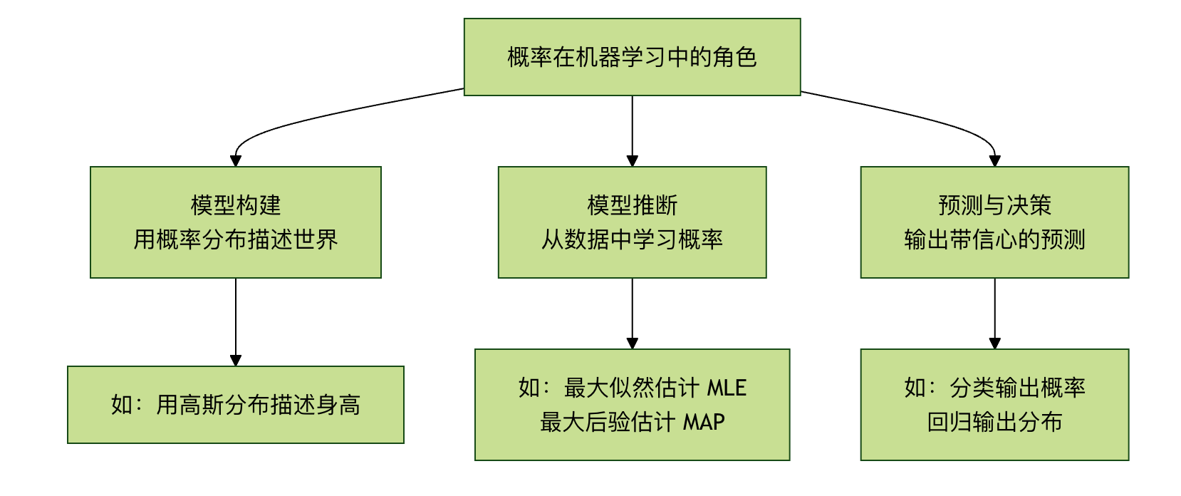
Role 1: Model Construction — Describing the World with Probability
Many machine learning models are essentiallyprobabilistic models. We assume that the observed data is generated by some underlying probability distribution.
Example 1: Logistic RegressionIt directly outputs a probability value. For a binary classification problem (cat/dog), the logistic regression model doesn't just say "this is a cat"; instead, it outputsP(类别=猫 | 图像数据)=0.9, indicating that the model has 90% confidence that this is a cat.
Example 2: Naive Bayes ClassifierIt directly applies Bayes' theorem for classification. It assumes that features are independent of each other, and calculatesP(垃圾邮件 | 词1, 词2...), then selects the category with the higher probability.
Example
# Assume we have estimated the following probabilities from the data (likelihoods and priors)
P_word_given_spam= {"free": 0.8, "meeting": 0.1} # The probability of "free" appearing in spam
P_word_given_normal= {"free": 0.1, "meeting": 0.9} # The probability of "meeting" appearing in normal emails
P_garbage= 0.3 # Prior probability: the probability that any email is spam
P_normal= 0.7 # Prior probability: the probability that any email is normal
# For an email containing "free" and "meeting", compute the posterior probability that it is spam (simplified calculation)
# According to Bayes' theorem (ignore the evidence denominator, as it cancels out when comparing)
score_spam=P_word_given_spam["free"]* P_word_given_spam["meeting"]* P_spam
score_normal=P_word_given_normal["free"]* P_word_given_normal["meeting"]* P_normal
print(f"Spam score: {score_垃圾:.4f}")
print(fNormal email score: {score_normal:.4f})
ifscore_spam>score_normal:
print("Prediction: This is a spam email.")
else:
print("Prediction: This is a normal email.")
Role 2: Model Inference and Learning — Finding the Most Likely Explanation
How do we find, from the data, the probabilistic model most likely to have generated this data (i.e., learning model parameters)? Here are two core ideas:
1. Maximum Likelihood Estimation Core idea: Find the model parameters that make theprobability of observing the current data(the likelihood) maximized.Analogy: A detective solving a case. The detective asks: "Under which motive and method would it be most likely to produce all the crime scene traces we currently see?" MLE is exactly about finding this "most likely" hypothesis.Advantages: Data-driven, relying completely on the data.Potential disadvantages: If the amount of data is small, it may overfit; it ignores prior knowledge.
2. Maximum A Posteriori Estimation
Core idea: Building on maximum likelihood, it incorporates ourprior knowledge of the parameters(P(假设)), and finds the parameters that maximize the posterior probability.Analogy: An experienced detective solving a case. He not only examines the crime scene traces (data), but also combines the suspect's known modus operandi (prior) to make a comprehensive judgment.Advantages: It can leverage domain knowledge, performs more robustly on small datasets, and prevents overfitting.
| Criterion | Full name | Optimization objective | Core idea | Vivid analogy |
|---|---|---|---|---|
| MLE | Maximum Likelihood Estimation | Maximize P(data | parameters) | Data-driven: Given the observed data, find the model parameters most likely to have generated that data. | Detective solving a case: identifying a suspect solely based on crime scene evidence |
| MAP | Maximum a posteriori estimation | Maximize P(parameters | data) | Prior + data: Combine prior knowledge and observed data, calculate the posterior probability of the parameters and take the maximum | Judge deciding a case: making a judgment based on legal provisions (prior) and evidence (data) |
Role 3: Prediction and Decision-Making — Outputting Answers with Confidence
A good model should not only give predictions, but also providethe uncertainty of predictions。
- Classification tasks: Output the probability of each category (e.g., cat: 0.85, dog: 0.12, rabbit: 0.03). This contains more information than simply outputting "cat". We can make decisions based on probability thresholds (e.g., only adopt when the highest probability is > 0.8).
- Regression tasks: Advanced regression models (such as probabilistic regression, Bayesian linear regression) can predict adistribution(such as a Gaussian distribution), rather than just a point estimate. It will tell you: "The predicted price is 1 million yuan, and there is 95% confidence that the true price is between 950,000 and 1,050,000 yuan."
Part 3: Hands-On Practice — Solving a Simple Problem with Probabilistic Thinking
Scenario: A simple disease test. Given:
- The prevalence of the disease in the general population (prior probability)
P(病) = 0.001。 - The accuracy of the test: if the person is truly sick, the probability of testing positive
P(阳|病) = 0.99(sensitivity). If not sick, the probability of testing negativeP(阴|健康) = 0.99(specificity). - Question: If a person tests positive, the probability that they actually have the disease
P(病|阳)is what?
The Intuition Trap: Many people would think it is as high as 99%. Let us use Bayes' theorem to calculate.
Example
P_disease = 0.001 # P(disease)
P_positive_given_disease = 0.99 # P(positive|disease)
P_negative_given_healthy = 0.99 # P(negative|healthy)
# Calculate derived probabilities
P_healthy = 1 - P_disease # P(healthy)
P_positive_given_healthy = 1 - P_negative_given_healthy # P(positive|healthy) = 1 - specificity
# Calculate the total probability P(positive)
# P(positive) = P(positive|disease)*P(disease) + P(positive|healthy)*P(healthy)
P_positive = (P_positive_given_disease * P_disease) + (P_positive_given_healthy * P_healthy)
# Apply Bayes' theorem to calculate P(disease|positive)
P_disease_given_positive = (P_positive_given_disease * P_disease) / P_positive
print(f"Even if the test is positive, the posterior probability of actually having the disease P(disease|positive) is only: {P_disease_given_positive:.2%}")
Running Results and Reflection:
You will be surprised to find thatP(病|阳)it is only about9%! This is because the disease prevalence is very low (low prior probability), resulting in far more false positives than true positives. This example profoundly demonstrates:
- The importance of prior knowledge: Ignoring the base rate can lead to serious misjudgment.
- The power of Bayesian reasoning: It forces us to take all relevant information (base rate, test accuracy) into consideration.
- The practicality of probabilistic thinking: It can correct systematic biases in our intuition.
Summary and Further Directions
Key Takeaways from Probabilistic Thinking:
- Embrace Uncertainty: The world is uncertain, and the output of models should also be probabilistic.
- Bayes is a Philosophy of Updating: Through the
Prior + Data -> Posteriorframework, continuously revise cognition with new evidence. - Decisions Require Probability: A good prediction should come with a "confidence score" to support decisions with controlled risk.
If you want to go deeper:
- Theoretical level: Studyprobabilistic graphical models, which elegantly represent complex probabilistic dependencies between variables using graph structures.
- Algorithmic level: Explorevariational inferenceandMarkov Chain Monte Carlomethods, which are powerful tools for solving complex Bayesian models.
- Application level: ResearchBayesian optimization(for hyperparameter tuning),Gaussian processes(for regression and optimization), anddeep generative models(such as variational autoencoders (VAE), diffusion models).