Titanic Survival Prediction
If you are just starting to learn machine learning, you might feel that those complex algorithms and mathematical formulas are far removed from the real world. But today, through a classic case — Titanic survival prediction — we will experience a complete machine learning project workflow firsthand.
The Titanic dataset is one of the most famous introductory projects in machine learning. It is based on real information about passengers during the sinking of the Titanic in 1912. Our goal is:Build a model to predict whether they survived the disaster, based on passengers' age, sex, ticket class, and other information.。
This project is classic because it perfectly covers the core steps of a machine learning project:
- Data Understanding and Exploration
- Data Cleaning and Preprocessing
- Feature Engineering
- Model Selection and Training
- Model Evaluation and Optimization
Through this hands-on case, you will no longer just read theory, but truly understand how to apply machine learning to solve real-world problems.
Step 1: Understand Our Data
Before writing any code, we must first understand the data at hand. The Titanic dataset typically contains the following fields (features):
| Field Name | Description | Data Type | Remarks |
|---|---|---|---|
PassengerId |
Passenger ID | Integer | Unique identifier, not helpful for prediction |
Survived |
Survived | Integer (0/1) | Target variable, 0=perished, 1=survived |
Pclass |
Ticket class (Pclass) | Integer (1,2,3) | 1=first class, 2=second class, 3=third class |
Name |
Passenger Name | String | Contains titles (e.g., Mr., Miss.), can extract new features |
Sex |
Sex | String | maleorfemale |
Age |
Age | Float | Has some missing values |
SibSp |
Number of siblings/spouses aboard | Integer | |
Parch |
Number of parents/children aboard | Integer | |
Ticket |
Ticket number | String | Complex structure, may have limited information |
Fare |
Fare | Float | |
Cabin |
Cabin | String | Many missing values, but the first letter may represent the cabin area |
Embarked |
Embarked (port of embarkation) | String | C=Cherbourg, Q=Queenstown, S=Southampton |
Key insight: From historical knowledge, we know that the "women and children first" principle was followed, and first-class passengers had priority access to lifeboats. Therefore, we expectSex, Age, Pclasssuch features will have a significant impact on the prediction results.
Step 2: Data Cleaning and Preprocessing
Raw data is almost never perfect.
Data cleaning is like preparing high-quality ingredients for the model; this step is crucial.
Save the following data to the train.csv file:
PassengerId,Survived,Pclass,Name,Sex,Age,SibSp,Parch,Ticket,Fare,Cabin,Embarked
1,0,3,"Braund, Mr. Owen Harris",male,22,1,0,A/5 21171,7.25,,S
2,1,1,"Cumings, Mrs. John Bradley",female,38,1,0,PC 17599,71.2833,C85,C
3,1,3,"Heikkinen, Miss. Laina",female,26,0,0,STON/O2. 3101282,7.925,,S
4,1,1,"Futrelle, Mrs. Jacques Heath",female,35,1,0,113803,53.1,C123,S
5,0,3,"Allen, Mr. William Henry",male,35,0,0,373450,8.05,,S
6,0,3,"Moran, Mr. James",male,,0,0,330877,8.4583,,Q
7,0,1,"McCarthy, Mr. Timothy J",male,54,0,0,17463,51.8625,E46,S
8,0,3,"Palsson, Master. Gosta Leonard",male,2,3,1,349909,21.075,,S
9,1,3,"Johnson, Mrs. Oscar W",female,27,0,2,347742,11.1333,,S
10,1,2,"Nasser, Mrs. Nicholas",female,14,1,0,237736,30.0708,,C
Save the following data to the test.csv file:
PassengerId,Pclass,Name,Sex,Age,SibSp,Parch,Ticket,Fare,Cabin,Embarked
11,3,"Kelly, Mr. James",male,34.5,0,0,330911,7.8292,,Q
12,3,"Wilkes, Mrs. James",female,47,1,0,363272,7,,S
13,2,"Myles, Mr. Thomas Francis",male,62,0,0,240276,9.6875,,Q
14,3,"Dwyer, Miss. Ellen",female,18,0,0,330959,7.75,,Q
15,1,"Jones, Mr. Charles",male,,1,0,PC 17603,82.1708,B28,C
We will use Python'spandasandnumpylibrary to accomplish this task.
Example
import pandas as pd
import numpy as np
# Load data
train_data = pd.read_csv('train.csv') # Training set, contains target variable Survived
test_data = pd.read_csv('test.csv') # Test set, does not contain Survived, used for final evaluation
# 1. Initial look at the data
print("Training set shape: ", train_data.shape)
print(train_data.info()) # Check data types and missing values
print(train_data.head()) # View the first few rows of data
Output:
训练集形状: (10, 12)
<class 'pandas.core.frame.DataFrame'>
RangeIndex: 10 entries, 0 to 9
Data columns (total 12 columns):
 #   Column       Non-Null Count  Dtype
---  ------       --------------  -----
 0   PassengerId  10 non-null     int64
 1   Survived     10 non-null     int64
 2   Pclass       10 non-null     int64
 3   Name         10 non-null     object
 4   Sex          10 non-null     object
 5   Age          9 non-null      float64
 6   SibSp        10 non-null     int64
 7   Parch        10 non-null     int64
 8   Ticket       10 non-null     object
 9   Fare         10 non-null     float64
 10  Cabin        3 non-null      object
 11  Embarked     10 non-null     object
dtypes: float64(2), int64(5), object(5)
memory usage: 1.1+ KB
None
   PassengerId  Survived  Pclass                          Name     Sex  ...  Parch            Ticket     Fare Cabin  Embarked
0            1         0       3       Braund, Mr. Owen Harris    male  ...      0         A/5 21171   7.2500   NaN         S
1            2         1       1    Cumings, Mrs. John Bradley  female  ...      0          PC 17599  71.2833   C85         C
2            3         1       3        Heikkinen, Miss. Laina  female  ...      0  STON/O2. 3101282   7.9250   NaN         S
3            4         1       1  Futrelle, Mrs. Jacques Heath  female  ...      0            113803  53.1000  C123         S
4            5         0       3      Allen, Mr. William Henry    male  ...      0            373450   8.0500   NaN         S

[5 rows x 12 columns]
After running the above code, you may find two main problems:Missing valuesandNon-numeric data。
Handling Missing Values
Example
print(train_data.isnull().sum())
# Handle Age: fill with median
train_data['Age'] = train_data['Age'].fillna(train_data['Age'].median())
test_data['Age'] = test_data['Age'].fillna(test_data['Age'].median())
# Handle Embarked: fill with mode
most_common_port = train_data['Embarked'].mode()[0]
train_data['Embarked'] = train_data['Embarked'].fillna(most_common_port)
test_data['Embarked'] = test_data['Embarked'].fillna(most_common_port)
# Handle Fare (ticket price): test set
test_data['Fare'] = test_data['Fare'].fillna(test_data['Fare'].median())
# Handle Cabin: drop directly
train_data.drop(columns=['Cabin'], inplace=True)
test_data.drop(columns=['Cabin'], inplace=True)
Converting Non-numeric Data
Machine learning models can usually only process numeric values. We need to convertSexandEmbarkedtext columns like this into numbers.
Example
train_data['Sex'] = train_data['Sex'].map({'female': 0, 'male': 1})
test_data['Sex'] = test_data['Sex'].map({'female': 0, 'male': 1})
# Convert Embarked column to numeric (One-Hot Encoding)
# Because ports have no order, simple mapping with 0,1,2 is not suitable
train_data = pd.get_dummies(train_data, columns=['Embarked'])
test_data = pd.get_dummies(test_data, columns=['Embarked'])
Step 3: Feature Engineering
Feature engineering is the "magic" in machine learning; it helps the model learn better by creating or transforming features. WeNameextracting "titles" from the column is a classic example.
Example
# Titles often reflect age, social status, and sex, and may affect rescue priority
train_data['Title'] = train_data['Name'].str.extract(' ([A-Za-z]+)\.', expand=False)
test_data['Title'] = test_data['Name'].str.extract(' ([A-Za-z]+)\.', expand=False)
# View the available titles
print(pd.crosstab(train_data['Title'], train_data['Sex']))
# Group uncommon titles into 'Rare'
title_mapping = {
'Mr': 'Mr', 'Miss': 'Miss', 'Mrs': 'Mrs',
'Master': 'Master', 'Dr': 'Rare', 'Rev': 'Rare',
'Col': 'Rare', 'Major': 'Rare', 'Mlle': 'Miss',
'Countess': 'Rare', 'Ms': 'Miss', 'Lady': 'Rare',
'Jonkheer': 'Rare', 'Don': 'Rare', 'Dona': 'Rare',
'Mme': 'Mrs', 'Capt': 'Rare', 'Sir': 'Rare'
}
train_data['Title'] = train_data['Title'].map(title_mapping)
test_data['Title'] = test_data['Title'].map(title_mapping)
# One-hot encode the processed Title column as well
train_data = pd.get_dummies(train_data, columns=['Title'])
test_data = pd.get_dummies(test_data, columns=['Title'])
# Create new feature: family size
train_data['FamilySize'] = train_data['SibSp'] + train_data['Parch'] + 1
test_data['FamilySize'] = test_data['SibSp'] + test_data['Parch'] + 1
# Create new feature: is alone
train_data['IsAlone'] = (train_data['FamilySize'] == 1).astype(int)
test_data['IsAlone'] = (test_data['FamilySize'] == 1).astype(int)
# Drop original columns that are no longer needed
columns_to_drop = ['PassengerId', 'Name', 'Ticket', 'SibSp', 'Parch']
train_data.drop(columns_to_drop, axis=1, inplace=True)
test_passenger_ids = test_data['PassengerId'] # Save test set IDs for later submission
test_data.drop(columns_to_drop, axis=1, inplace=True)
print("Training set column names after feature engineering: ", train_data.columns.tolist())
Step 4: Selecting and Training the Model
Now we have clean and informative numeric data. Next, we split it intofeatures (X)andtarget variable (y), and then select a model to train.
We will start with a simple and efficientRandom Forestmodel.
Example
from sklearn.model_selection import train_test_split
from sklearn.ensemble import RandomForestClassifier
from sklearn.metrics import accuracy_score
# Prepare data
# X is the feature matrix, y is the target vector we want to predict
X = train_data.drop('Survived', axis=1)
y = train_data['Survived']
# To evaluate model performance during training, we split the data into training and validation sets
# test_size=0.2 means 20% of the data is used for validation, 80% for training
# random_state is a random seed to ensure consistent split results each time
X_train, X_val, y_train, y_val = train_test_split(X, y, test_size=0.2, random_state=42)
# Initialize the Random Forest classifier
# n_estimators: number of trees in the forest
# max_depth: maximum depth of trees, controls model complexity, prevents overfitting
# random_state: ensures reproducible results
model = RandomForestClassifier(n_estimators=100, max_depth=5, random_state=42)
# Train the model (let the model learn patterns from the data)
model.fit(X_train, y_train)
# Make predictions on the validation set
y_pred = model.predict(X_val)
# Evaluate model accuracy
accuracy = accuracy_score(y_val, y_pred)
print(f"The model's accuracy on the validation set is: {accuracy:.4f} (i.e., {accuracy*100:.2f}%)")
Step 5: Model Evaluation, Optimization, and Submission
Evaluation and Optimization
The result of a single training run may not be optimal. We can improve it in the following ways:
- Tune model parameters: for example, try different
n_estimatorsormax_depth。 - Try other models: such as logistic regression, support vector machines, gradient boosting trees, etc.
- Further feature engineering: for example, for
AgeorFareperform binning.
Example
for depth in [3, 5, 10, None]: # None means no depth limit
model_temp = RandomForestClassifier(n_estimators=100, max_depth=depth, random_state=42)
model_temp.fit(X_train, y_train)
y_pred_temp = model_temp.predict(X_val)
acc = accuracy_score(y_val, y_pred_temp)
print(f"When max_depth={depth}, validation set accuracy: {acc:.4f}")
Feature Importance Analysis
Random Forest can tell us which features contribute the most to predictions.
Example
feature_importances = pd.DataFrame({
'feature': X_train.columns,
'importance': model.feature_importances_
}).sort_values('importance', ascending=False)
print("Feature importance ranking:")
print(feature_importances)
You may findSex, Fare(relatedPclass), Age, Titleis the most important feature, which aligns with our historical intuition.
Generating Final Predictions on the Test Set
Once we are satisfied with the model's performance, we retrain on the full training data and make predictions on the actual test set.
Example
final_model = RandomForestClassifier(n_estimators=100, max_depth=5, random_state=42)
final_model.fit(X, y) # This time use all training data X, y
# Ensure the test set's feature columns are exactly the same as the training set (order and number of columns)
# pd.get_dummies may lead to different numbers of columns in training and test sets (if a category appears only in one side)
# Here we need to align columns. A simple way is to merge and then split, but a more robust approach is to ensure encoding consistency.
# For simplicity, assume the processed test set columns are aligned.
final_predictions = final_model.predict(test_data)
# Create submission file
submission = pd.DataFrame({
'PassengerId': test_passenger_ids,
'Survived': final_predictions
})
submission.to_csv('my_titanic_submission.csv', index=False)
print(The prediction results have been saved to 'my_titanic_submission.csv'. You can submit them to the Kaggle platform to view the ranking!)
Summary and Project Flowchart
We have completed a full machine learning pipeline. Let's review the entire process with a flowchart:
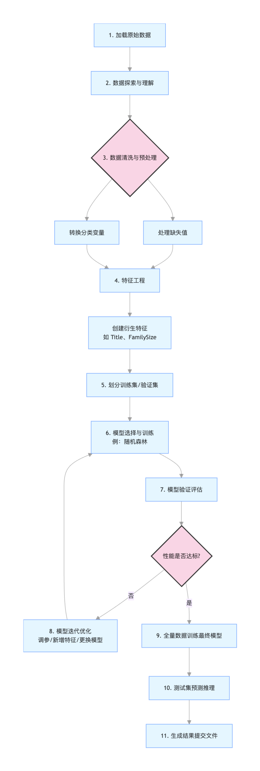
Through this hands-on project, you not only learnedpandasperforming data processing,sklearnthe techniques for building models, but more importantly, you masteredthe standard approach to solving a machine learning problem.。
This workflow—from data understanding to model deployment—is the core of the vast majority of data science projects.
other extensions