Machine Learning Basic Terminology
Learning machine learning is like learning a new language; you need to master the basic vocabulary first. These terms form the "language system" of machine learning, and understanding them is the first step toward deeper learning.
Imagine you are teaching a robot to recognize fruits:
- Data: Images and information of various fruits
- Feature: The color, shape, size, and taste of the fruit
- Label: The name of this fruit (apple, banana, orange)
- Model: The "method of recognizing fruits" learned by the robot
- Training: The process of teaching the robot to recognize fruits
- Inference: The robot's ability to recognize new fruits
Data
What is Data?
Datais the "raw material" of machine learning, just like ingredients a chef needs to cook. Without data, machine learning cannot proceed.

Types of Data
1. Structured Data
Characteristics: Has a clear format and organization, neat like a table
# Structured data example: Student information tableExample
students_data = {
'Name': ['Zhang San', 'Li Si', 'Wang Wu'],
'Age': [18, 19, 20],
'Score': [85, 92, 78],
'Class': ['Class 1', 'Class 2', 'Class 1']
}
df = pd.DataFrame(students_data)
print(df)
Output:
   姓名  年龄  成绩  班级
0  张三  18  85  一班
1  李四  19  92  二班
2  王五  20  78  一班
2. Unstructured Data
Characteristics: Has no fixed format and requires special processing
Examples:
- Text: comments, articles, emails
- Images: photos, medical images
- Audio: speech, music
- Video: surveillance footage, movies
# 非结构化数据示例:文本和图像
text_data = "这个产品质量很好,我很满意!"
# image_data = 一张产品的照片
# audio_data = 顾客的语音评价
Importance of Data Quality
Garbage in, garbage out(Garbage In, Garbage Out) is an important principle of machine learning. Data quality directly determines model performance.
Example
import numpy as np
import pandas as pd
# Create data with various issues
problematic_data = {
'Price': [100, 200, None, 300, -50], # Missing values and outliers
'Rating': [4.5, 'Good', 3.8, 4.2, 5.0], # Inconsistent data types
'Sales': [1000, 1200, 800, 1500, 'Many'] # Mixture of text and numbers
}
df = pd.DataFrame(problematic_data)
print("Problematic data:")
print(df)
print("\nData issue analysis: ")
print(f"Number of missing values: {df.isnull().sum().sum()}")
print(f"Data types:\n{df.dtypes}")
Feature
What is a Feature?
Featureis an "observable attribute" of data, just like describing a person's characteristics: height, weight, hair color, personality, etc. In machine learning, features are the basis for making predictions.
Importance of Feature Selection:
- Good features can make the model twice as effective with half the effort
- Bad features can make the model half as effective with twice the effort
- Feature engineering is often the key to determining model performance
Types of Features
1. Numerical Features
Characteristics: Can be represented by numbers and can undergo mathematical operations
# 数值特征示例
numerical_features = {
    '年龄': [25, 30, 35, 40],
    '收入': [5000, 8000, 12000, 15000],
    '身高': [165, 170, 175, 180]
}
2. Categorical Features
Characteristics: Represents different categories and cannot undergo mathematical operations
# 类别特征示例
categorical_features = {
    '性别': ['男', '女', '男', '女'],
    '学历': ['本科', '硕士', '博士', '本科'],
    '城市': ['北京', '上海', '广州', '深圳']
}
3. Text Features
Characteristics: Requires special processing before it can be used by the model
# 文本特征示例
text_features = {
    '评论': [
        '这个产品很好用,推荐购买!',
        '质量一般,不太满意。',
        '性价比高,值得入手。'
    ]
}
Feature Engineering Example
Example
import pandas as pd
import numpy as np
# Raw data: house information
house_data = {
'Area': [80, 120, 60, 150, 90],
'Number of Bedrooms': [2, 3, 1, 4, 2],
'Year Built': [2000, 2010, 1995, 2015, 2005],
'Price': [200, 350, 150, 500, 280]
}
df = pd.DataFrame(house_data)
# Create new features
df['House Age'] = 2023 - df['Year Built'] # House age
df['Price per Square Meter'] = df['Price'] / df['Area'] # Unit price
df['Bedroom Area Ratio'] = df['Number of Bedrooms'] / df['Area'] * 100 # Bedroom ratio
print("Raw data + new features:")
print(df)
# Feature importance analysis
correlation = df.corr()['Price'].sort_values(ascending=False)
print("\nCorrelation between features and price: ")
print(correlation)
Label
What is a Label?
Labelis the "answer" we want to predict, just like the correct answer to an exam question. In supervised learning, each data sample has a corresponding label.
Role of Labels:
- Guide the model's learning direction
- Evaluate the model's learning effectiveness
- Define the type of problem
Types of Labels
1. Classification Labels
Characteristics: Discrete categorical values
# 分类标签示例
classification_labels = {
    '邮件类型': ['垃圾邮件', '正常邮件', '垃圾邮件', '正常邮件'],
    '情感倾向': ['正面', '负面', '中性', '正面'],
    '疾病诊断': ['患病', '健康', '健康', '患病']
}
2. Regression Labels
Characteristics: Continuous numerical values
# 回归标签示例
regression_labels = {
    '房价': [250000, 320000, 180000, 450000],
    '温度': [25.5, 28.3, 22.1, 30.0],
    '股票价格': [100.5, 105.2, 98.7, 110.3]
}
Importance of Label Quality
# 标签质量问题示例
import numpy as np
# 模拟图像分类任务中的标签问题
image_data = ['cat1.jpg', 'dog1.jpg', 'cat2.jpg', 'dog2.jpg']
problematic_labels = ['猫', '犬', '猫咪', '狗']  # 标签不一致
# 标签标准化
label_mapping = {
    '猫': 'cat', '猫咪': 'cat',
    '犬': 'dog', '狗': 'dog'
}
standardized_labels = [label_mapping[label] for label in problematic_labels]
print("原始标签:", problematic_labels)
print("标准化标签:", standardized_labels)
Model
What is a Model?
Modelis the "pattern" or "rule" that a machine learning algorithm learns from data, just like the knowledge students learn from textbooks.
Essence of a Model:
- Mathematical function: input features, output predictions
- Set of parameters: concrete representation of the learned rules
- Decision rules: how to get output from input
Representation of a Model
Example
import numpy as np
import matplotlib.pyplot as plt
# Simulated data
X = np.array([1, 2, 3, 4, 5])
y = np.array([2, 4, 6, 8, 10])
# Linear model: y = w * x + b
# Learned parameters: w = 2, b = 0
w, b = 2, 0
def linear_model(x):
"""Linear model function"""
return w * x + b
# Prediction
predictions = linear_model(X)
# Visualization
plt.scatter(X, y, color='blue', label='True data')
plt.plot(X, predictions, color='red', label='Model predictions')
plt.xlabel('Input X')
plt.ylabel('Output y')
plt.title('Linear model example')
plt.legend()
plt.grid(True)
plt.show()
print(f"Model parameters: w = {w}, b = {b}")
print(f"Prediction results: {predictions}")
Model Complexity
Example
from sklearn.preprocessing import PolynomialFeatures
from sklearn.linear_model import LinearRegression
import numpy as np
# Generate nonlinear data
np.random.seed(42)
X = np.random.rand(20, 1) * 10
y = np.sin(X) + np.random.randn(20, 1) * 0.1
# Simple model (linear)
simple_model = LinearRegression()
simple_model.fit(X, y)
# Complex model (high-degree polynomial)
poly_features = PolynomialFeatures(degree=10)
X_poly = poly_features.fit_transform(X)
complex_model = LinearRegression()
complex_model.fit(X_poly, y)
# Visualization
X_test = np.linspace(0, 10, 100).reshape(-1, 1)
X_test_poly = poly_features.transform(X_test)
plt.scatter(X, y, color='blue', label='Training data')
plt.plot(X_test, simple_model.predict(X_test), color='green', label='Simple model')
plt.plot(X_test, complex_model.predict(X_test_poly), color='red', label='Complex model')
plt.xlabel('X')
plt.ylabel('y')
plt.title('Model complexity comparison')
plt.legend()
plt.grid(True)
plt.show()
Training
What is Training?
Trainingis the process by which a model learns, just like students learning knowledge in class. During training, the model continuously adjusts its parameters so that predictions get closer and closer to the true labels.
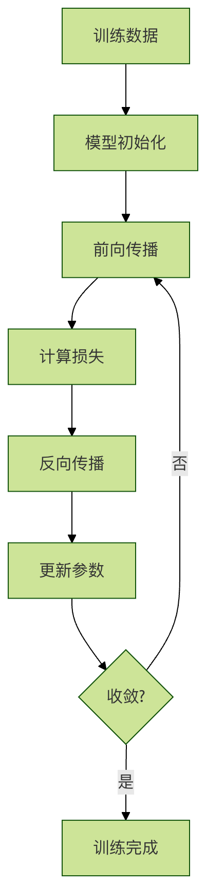
Training Process Example
Example
import numpy as np
import matplotlib.pyplot as plt
# Generate training data
np.random.seed(42)
X = np.random.rand(50, 1) * 10
y = 3 * X + 2 + np.random.randn(50, 1) * 2
# Initialize model parameters
w, b = 0.0, 0.0
learning_rate = 0.01
epochs = 100
# Record the training process
loss_history = []
# Training loop
for epoch in range(epochs):
# Forward propagation
y_pred = w * X + b
# Calculate loss (mean squared error)
loss = np.mean((y_pred - y) ** 2)
loss_history.append(loss)
# Calculate gradients
dw = np.mean(2 * X * (y_pred - y))
db = np.mean(2 * (y_pred - y))
# Update parameters
w -= learning_rate * dw
b -= learning_rate * db
if epoch % 10 == 0:
print(f"Epoch {epoch}: Loss = {loss:.4f}, w = {w:.4f}, b = {b:.4f}")
# Visualize the training process
plt.figure(figsize=(12, 4))
plt.subplot(1, 2, 1)
plt.plot(loss_history)
plt.xlabel('Epoch')
plt.ylabel('Loss')
plt.title('Training loss change')
plt.grid(True)
plt.subplot(1, 2, 2)
plt.scatter(X, y, color='blue', label='Training data')
plt.plot(X, w * X + b, color='red', label='Trained model')
plt.xlabel('X')
plt.ylabel('y')
plt.title('Training results')
plt.legend()
plt.grid(True)
plt.tight_layout()
plt.show()
print(f"Final model parameters: w = {w:.4f}, b = {b:.4f}")
Inference
What is Inference?
InferenceInference is the process of using a trained model to make predictions, just like students using learned knowledge to answer exam questions.
Inference Process Example
Example
import numpy as np
# Assume we have already trained a house price prediction model
class HousePriceModel:
def __init__(self):
# Simulate trained parameters
self.feature_weights = {
'Area': 2.5,
'Bedrooms': 10.0,
'House age': -1.0,
'Location score': 50.0
}
self.bias = 50.0
def predict(self, features):
"""
Use the trained model for house price prediction
"""
price = self.bias
for feature_name, feature_value in features.items():
if feature_name in self.feature_weights:
price += self.feature_weights[feature_name] * feature_value
return price
# Create the trained model
model = HousePriceModel()
# Inference: Predict new house price
new_houses = [
{'Area': 80, 'Bedrooms': 2, 'House age': 5, 'Location score': 8},
{'Area': 120, 'Bedrooms': 3, 'House age': 2, 'Location score': 9},
{'Area': 60, 'Bedrooms': 1, 'House age': 10, 'Location score': 6}
]
print(House price prediction results:)
for i, house in enumerate(new_houses, 1):
predicted_price = model.predict(house)
print(f"House {i}: predicted price {predicted_price:.2f} ten thousand yuan")
# Batch inference
def batch_predict(model, house_list):
"""Batch prediction"""
return [model.predict(house) for house in house_list]
batch_prices = batch_predict(model, new_houses)
print(f"\nBatch prediction results: {batch_prices}")
Complete Example: From Data to Inference
Example
import numpy as np
import pandas as pd
from sklearn.model_selection import train_test_split
from sklearn.linear_model import LinearRegression
from sklearn.metrics import mean_squared_error, r2_score
# 1. Data preparation
np.random.seed(42)
n_samples = 200
# Generate feature data
area = np.random.normal(100, 30, n_samples) # Area
bedrooms = np.random.randint(1, 5, n_samples) # Bedrooms
age = np.random.randint(0, 20, n_samples) # House age
location_score = np.random.randint(1, 10, n_samples) # Location score
# Generate labels (house prices) - linear combination of features plus noise
price = (area * 2.5 + bedrooms * 20 + age * -2 + location_score * 15 +
np.random.normal(0, 50, n_samples))
# Create DataFrame
data = pd.DataFrame({
'Area': area,
'Bedrooms': bedrooms,
'House age': age,
'Location score': location_score,
'Price': price
})
print(Data example:)
print(data.head())
# 2. Split into training set and test set
features = ['Area', 'Bedrooms', 'House age', 'Location score']
X = data[features]
y = data['Price']
X_train, X_test, y_train, y_test = train_test_split(X, y, test_size=0.2, random_state=42)
print(f"\nTraining set size: {X_train.shape)
print(f"Test set size: {X_test.shape)
# 3. Train the model
model = LinearRegression()
model.fit(X_train, y_train)
print(f"\nModel parameters:")
for feature, coef in zip(features, model.coef_):
print(f"{feature}: {coef:.2f}")
print(f"Intercept: {model.intercept_:.2f}")
# 4. Evaluate the model
y_train_pred = model.predict(X_train)
y_test_pred = model.predict(X_test)
train_mse = mean_squared_error(y_train, y_train_pred)
test_mse = mean_squared_error(y_test, y_test_pred)
train_r2 = r2_score(y_train, y_train_pred)
test_r2 = r2_score(y_test, y_test_pred)
print(f"\nModel evaluation:")
print(f"Training set MSE: {train_mse:.2f}, R²: {train_r2:.2f}")
print(f"Test set MSE: {test_mse:.2f}, R²: {test_r2:.2f}")
# 5. Inference (predict new data)
new_houses = pd.DataFrame({
'Area': [85, 120, 65],
'Bedrooms': [2, 3, 1],
'House age': [3, 1, 8],
'Location score': [7, 9, 5]
})
predictions = model.predict(new_houses)
print(f"\nNew house price prediction:")
for i, price in enumerate(predictions, 1):
print(f"House {i}: {price:.2f} ten thousand yuan")
Common Machine Learning Network Types
| Model type | Chinese full name | English abbreviation | Core applicable scenarios | Advantages | Disadvantages |
|---|---|---|---|---|---|
| Traditional machine learning | Decision Tree | DT | Classification, regression, feature importance analysis | Strong interpretability, no data normalization required | Prone to overfitting, sensitive to noise |
| Random Forest | RF | Classification, regression, anomaly detection | Resistant to overfitting, high stability | High computational cost with high-dimensional data | |
| Logistic Regression | LR | Binary classification, probability prediction | Fast training, strong interpretability | Difficult to fit nonlinear relationships | |
| Support Vector Machine | SVM | Classification, high-dimensional small-sample data | Strong generalization ability, suitable for scenarios with high feature dimensions | Slow training on large-scale data, complex parameter tuning | |
| Naive Bayes | NB | Text classification, spam detection | Extremely fast training, insensitive to missing data | Assumes feature independence, which may not hold in real scenarios | |
| XGBoost | XGBoost | Classification, regression, competition-level tasks | High accuracy, supports parallel computing, built-in regularization | Prone to overfitting, sensitive to hyperparameters | |
| LightGBM | LightGBM | Large-scale data classification, regression | Fast training speed, low memory usage | May be less stable than XGBoost on small datasets | |
| Deep learning | Artificial Neural Network | ANN | Simple classification, regression tasks | Simple structure, easy to understand | Difficult to handle high-dimensional, complex data |
| Convolutional Neural Network | CNN | Image recognition, object detection, video analysis | Automatically extracts spatial features, parameter sharing | Training requires large amounts of data and computational resources | |
| Recurrent Neural Network | RNN | Sequence data processing, text generation | Handles variable-length sequences | Has vanishing/exploding gradient problems, difficult to capture long-term dependencies | |
| Long Short-Term Memory | LSTM | Long-sequence text translation, speech recognition | Solves RNN's long-dependency problem | Complex structure, relatively slow training speed | |
| Gated Recurrent Unit | GRU | Sequence data processing, sentiment analysis | Simpler structure than LSTM, faster training | Slightly inferior to LSTM in long-sequence scenarios | |
| Generative Adversarial Network | GAN | Image generation, style transfer, data augmentation | High quality generated data, strong diversity | Unstable training, prone to mode collapse | |
| Transformer | Transformer | Natural language processing, multimodal tasks | High parallel computing efficiency, strong ability to capture long dependencies | High computational cost, prone to overfitting on small datasets | |
| Autoencoder | AE | Data compression, anomaly detection, feature extraction | Unsupervised learning, simple structure | Generated data quality is usually lower than GAN | |
| Graph Neural Network | GNN | Social network analysis, molecular structure prediction | Processes graph-structured data, mines node relationships | Difficult to train, high requirements for graph structure preprocessing |