TensorFlow Examples - Regression Problems
What is a regression problem?
Regression problems are an important class of problems in machine learning whose goal is to predict continuous-valued outputs. Unlike classification problems (predicting discrete categories), regression problems predict numerical values within the real-number range.
Common examples of regression problems
- House price prediction: predict price based on features such as house area and location
- Stock prediction: predict future stock prices based on historical data
- Temperature prediction: predict future temperature based on meteorological data
Basic workflow of solving regression problems with TensorFlow
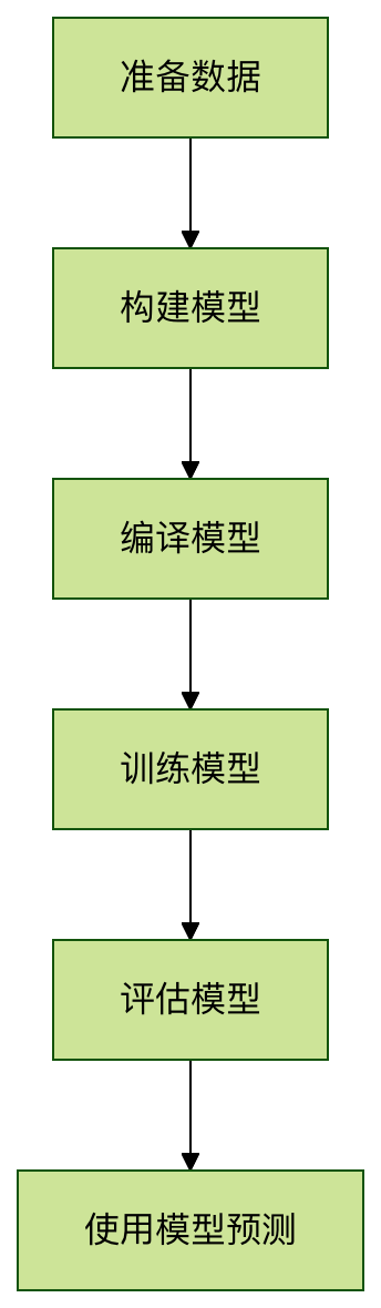
Hands-on: Boston housing price prediction
1. Prepare the data
We will use the classic Boston housing price dataset, which contains 506 samples, each with 13 features:
Example
from tensorflow.keras.datasets import boston_housing
# Load data
(train_data, train_targets), (test_data, test_targets) = boston_housing.load_data()
# Data standardization (important step)
mean = train_data.mean(axis=0)
train_data -= mean
std = train_data.std(axis=0)
train_data /= std
test_data -= mean
test_data /= std
# Load data
(train_data, train_targets), (test_data, test_targets) = boston_housing.load_data()
# Data standardization (important step)
mean = train_data.mean(axis=0)
train_data -= mean
std = train_data.std(axis=0)
train_data /= std
test_data -= mean
test_data /= std
2. Build the model
Example
from tensorflow.keras import models
from tensorflow.keras import layers
def build_model():
model = models.Sequential([
layers.Dense(64, activation='relu', input_shape=(train_data.shape[1],)),
layers.Dense(64, activation='relu'),
layers.Dense(1) # The output layer does not need an activation function
])
return model
from tensorflow.keras import layers
def build_model():
model = models.Sequential([
layers.Dense(64, activation='relu', input_shape=(train_data.shape[1],)),
layers.Dense(64, activation='relu'),
layers.Dense(1) # The output layer does not need an activation function
])
return model
Model structure description
- Input layer: corresponds to 13 features
- Two hidden layers: 64 neurons per layer, using ReLU activation function
- Output layer: 1 neuron (predict housing price), without activation function
3. Compile the model
Example
model = build_model()
model.compile(optimizer='rmsprop',
loss='mse', # Mean Squared Error
metrics=['mae']) # Mean Absolute Error
model.compile(optimizer='rmsprop',
loss='mse', # Mean Squared Error
metrics=['mae']) # Mean Absolute Error
Key parameter description
- optimizer: optimizer, controls the learning process
rmsprop: default choice suitable for most problems
- loss: loss function, commonly used in regression problems
mse(Mean Squared Error): Mean Squared Error
- metrics: evaluation metric
mae(Mean Absolute Error): Mean Absolute Error
4. Train the model
Example
history = model.fit(train_data, train_targets,
epochs=100,
batch_size=16,
validation_split=0.2)
epochs=100,
batch_size=16,
validation_split=0.2)
Parameter explanation
epochs: number of training epochsbatch_size: batch sizevalidation_split: validation split ratio
5. Evaluate the model
Example
# Evaluate on the test set
test_mse_score, test_mae_score = model.evaluate(test_data, test_targets)
print(f"Test set MAE: {test_mae_score}")
test_mse_score, test_mae_score = model.evaluate(test_data, test_targets)
print(f"Test set MAE: {test_mae_score}")
Understanding the evaluation metrics
- MAE (Mean Absolute Error): the average difference between predicted and true values
- For example, MAE=2.5 means the prediction deviates by an average of $25,000
- MSE (Mean Squared Error): gives greater penalty to larger errors
6. Use the model for prediction
Example
# Make predictions on new data
sample = test_data[0] # Take the first sample from the test set
prediction = model.predict(sample.reshape(1, -1))
print(f"Predicted price: {prediction)
sample = test_data[0] # Take the first sample from the test set
prediction = model.predict(sample.reshape(1, -1))
print(f"Predicted price: {prediction)
Model optimization techniques
1. Adjust the network structure
Example
# A deeper network may perform better
def build_deeper_model():
model = models.Sequential([
layers.Dense(128, activation='relu', input_shape=(train_data.shape[1],)),
layers.Dense(64, activation='relu'),
layers.Dense(32, activation='relu'),
layers.Dense(1)
])
return model
def build_deeper_model():
model = models.Sequential([
layers.Dense(128, activation='relu', input_shape=(train_data.shape[1],)),
layers.Dense(64, activation='relu'),
layers.Dense(32, activation='relu'),
layers.Dense(1)
])
return model
2. Use K-fold cross-validation
Example
from sklearn.model_selection import KFold
k = 4
kf = KFold(n_splits=k)
for train_index, val_index in kf.split(train_data):
# Split into training and validation sets
partial_train_data = train_data[train_index]
partial_train_targets = train_targets[train_index]
val_data = train_data[val_index]
val_targets = train_targets[val_index]
# Train and evaluate the model
model = build_model()
model.fit(partial_train_data, partial_train_targets,
epochs=100, batch_size=16, verbose=0)
val_mse, val_mae = model.evaluate(val_data, val_targets, verbose=0)
print(f"Validation MAE: {val_mae}")
k = 4
kf = KFold(n_splits=k)
for train_index, val_index in kf.split(train_data):
# Split into training and validation sets
partial_train_data = train_data[train_index]
partial_train_targets = train_targets[train_index]
val_data = train_data[val_index]
val_targets = train_targets[val_index]
# Train and evaluate the model
model = build_model()
model.fit(partial_train_data, partial_train_targets,
epochs=100, batch_size=16, verbose=0)
val_mse, val_mae = model.evaluate(val_data, val_targets, verbose=0)
print(f"Validation MAE: {val_mae}")
3. Add regularization to prevent overfitting
Example
from tensorflow.keras import regularizers
model = models.Sequential([
layers.Dense(64, activation='relu',
kernel_regularizer=regularizers.l2(0.001),
input_shape=(train_data.shape[1],)),
layers.Dense(64, activation='relu',
kernel_regularizer=regularizers.l2(0.001)),
layers.Dense(1)
])
model = models.Sequential([
layers.Dense(64, activation='relu',
kernel_regularizer=regularizers.l2(0.001),
input_shape=(train_data.shape[1],)),
layers.Dense(64, activation='relu',
kernel_regularizer=regularizers.l2(0.001)),
layers.Dense(1)
])
Common problems and solutions
Problem 1: The model performance is unstable
- Cause: small amount of data or randomness in initialization
- Solution: increase the amount of data or use K-fold cross-validation
Problem 2: Low training error but high test error
- Cause: overfitting
- Solution: add a Dropout layer or L2 regularization
Problem 3: The predicted values deviate greatly from the actual values
- Cause: data not standardized or network structure unreasonable
- Solution: check the data preprocessing steps, adjust the depth and width of the network