TensorFlow Model Evaluation and Monitoring
1. Basic Concepts of Model Evaluation
In machine learning projects, model evaluation is a critical step for validating model performance. It helps us understand how the model performs in real-world scenarios and guides us in model optimization.
1.1 Why Do We Need Model Evaluation
- Performance verification: Confirm whether the model achieves the expected results
- Model selection: Compare the strengths and weaknesses of different models
- Parameter tuning: Guide the direction of hyperparameter adjustment
- Avoid overfitting: Detect whether the model is overfitting to the training data
1.2 Types of Evaluation Metrics
| Metric Type | Applicable Scenario | Common Metrics |
|---|---|---|
| Classification Metrics | Classification problems | Accuracy, precision, recall, F1 score |
| Regression Metrics | Regression problems | MSE、MAE、R² |
| Clustering Metrics | Unsupervised learning | Silhouette coefficient, Davies-Bouldin index |
2. TensorFlow Evaluation Tools
TensorFlow provides a variety of tools and methods to evaluate model performance.
2.1 Built-in Evaluation Metrics
Example
import tensorflow as tf
# Commonly used classification metrics
metrics = [
tf.keras.metrics.BinaryAccuracy(),
tf.keras.metrics.Precision(),
tf.keras.metrics.Recall(),
tf.keras.metrics.AUC()
]
# Commonly used regression metrics
metrics = [
tf.keras.metrics.MeanSquaredError(),
tf.keras.metrics.MeanAbsoluteError(),
tf.keras.metrics.RootMeanSquaredError()
]
# Commonly used classification metrics
metrics = [
tf.keras.metrics.BinaryAccuracy(),
tf.keras.metrics.Precision(),
tf.keras.metrics.Recall(),
tf.keras.metrics.AUC()
]
# Commonly used regression metrics
metrics = [
tf.keras.metrics.MeanSquaredError(),
tf.keras.metrics.MeanAbsoluteError(),
tf.keras.metrics.RootMeanSquaredError()
]
2.2 Evaluation Process
1. Specify metrics when compiling the model
Example
model.compile(
optimizer='adam',
loss='binary_crossentropy',
metrics=['accuracy', tf.keras.metrics.AUC()]
)
optimizer='adam',
loss='binary_crossentropy',
metrics=['accuracy', tf.keras.metrics.AUC()]
)
2. Use the evaluate method for evaluation
Example
test_loss, test_acc, test_auc = model.evaluate(
test_images, test_labels, verbose=2
)
test_images, test_labels, verbose=2
)
3. Custom evaluation functions
Example
import tensorflow as tf
@tf.function
def custom_metric(y_true, y_pred):
threshold = 0.5
y_pred = tf.cast(y_pred > threshold, tf.float32)
# Calculate accuracy, not just the proportion of positive examples
correct_predictions = tf.cast(tf.equal(y_true, y_pred), tf.float32)
return tf.reduce_mean(correct_predictions)
model.compile(
optimizer='adam',
loss='binary_crossentropy',
metrics=[custom_metric, 'accuracy'] # You can also keep the standard accuracy metric as a reference
)
@tf.function
def custom_metric(y_true, y_pred):
threshold = 0.5
y_pred = tf.cast(y_pred > threshold, tf.float32)
# Calculate accuracy, not just the proportion of positive examples
correct_predictions = tf.cast(tf.equal(y_true, y_pred), tf.float32)
return tf.reduce_mean(correct_predictions)
model.compile(
optimizer='adam',
loss='binary_crossentropy',
metrics=[custom_metric, 'accuracy'] # You can also keep the standard accuracy metric as a reference
)
3. Model Monitoring and Visualization
1. TensorBoard Integration
TensorBoard is TensorFlow's visualization tool that allows real-time monitoring of the training process.
Example
# Set up the callback function
tensorboard_callback = tf.keras.callbacks.TensorBoard(
log_dir='./logs',
histogram_freq=1,
write_graph=True,
write_images=True
)
# Add the callback when training the model
model.fit(
train_data,
epochs=10,
validation_data=val_data,
callbacks=[tensorboard_callback]
)
tensorboard_callback = tf.keras.callbacks.TensorBoard(
log_dir='./logs',
histogram_freq=1,
write_graph=True,
write_images=True
)
# Add the callback when training the model
model.fit(
train_data,
epochs=10,
validation_data=val_data,
callbacks=[tensorboard_callback]
)
Launch TensorBoard:
tensorboard --logdir=./logs
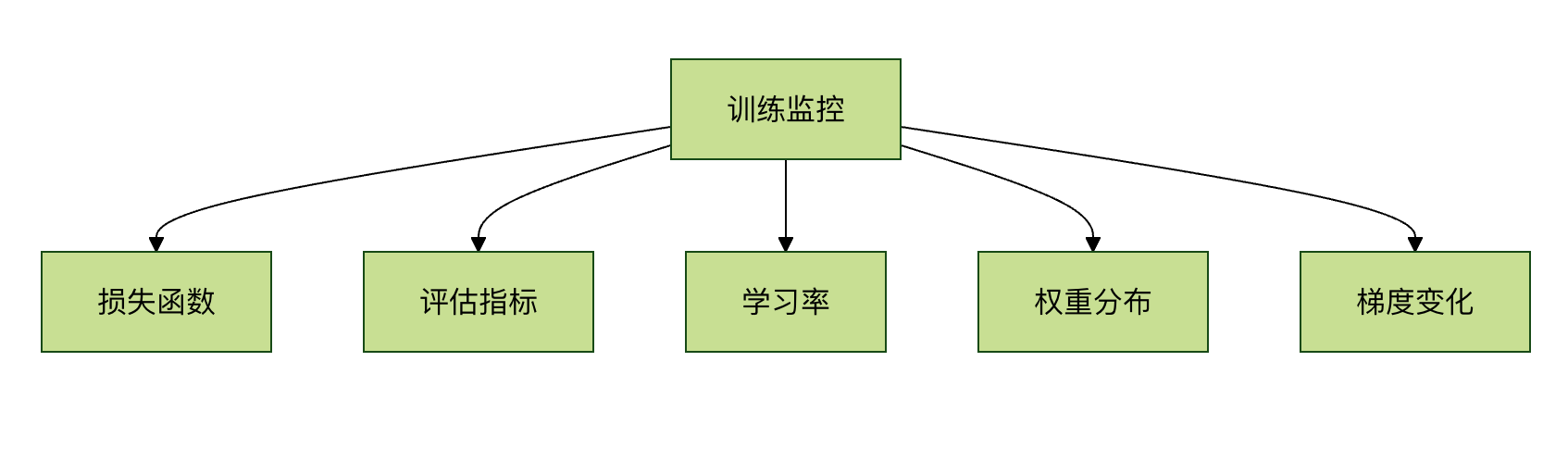
2. Key Metrics for Monitoring
4. Advanced Evaluation Techniques
4.1 Cross-Validation
Example
from sklearn.model_selection import KFold
import numpy as np
# Prepare data
X = np.array(...)
y = np.array(...)
# 5-fold cross-validation
kfold = KFold(n_splits=5, shuffle=True)
fold_no = 1
for train, test in kfold.split(X, y):
# Create model
model = create_model()
# Train model
model.fit(X[train], y[train], epochs=10)
# Evaluate model
scores = model.evaluate(X[test], y[test])
print(f'Fold {fold_no} - {model.metrics_names[0]}: {scores[0]}')
fold_no += 1
import numpy as np
# Prepare data
X = np.array(...)
y = np.array(...)
# 5-fold cross-validation
kfold = KFold(n_splits=5, shuffle=True)
fold_no = 1
for train, test in kfold.split(X, y):
# Create model
model = create_model()
# Train model
model.fit(X[train], y[train], epochs=10)
# Evaluate model
scores = model.evaluate(X[test], y[test])
print(f'Fold {fold_no} - {model.metrics_names[0]}: {scores[0]}')
fold_no += 1
4.2 Confusion Matrix Analysis
Example
from sklearn.metrics import confusion_matrix
import seaborn as sns
import matplotlib.pyplot as plt
# Get prediction results
y_pred = model.predict(test_images)
y_pred_classes = np.argmax(y_pred, axis=1)
# Generate confusion matrix
conf_mat = confusion_matrix(test_labels, y_pred_classes)
# Visualization
plt.figure(figsize=(10, 8))
sns.heatmap(conf_mat, annot=True, fmt='d')
plt.xlabel('Predicted')
plt.ylabel('Actual')
plt.show()
import seaborn as sns
import matplotlib.pyplot as plt
# Get prediction results
y_pred = model.predict(test_images)
y_pred_classes = np.argmax(y_pred, axis=1)
# Generate confusion matrix
conf_mat = confusion_matrix(test_labels, y_pred_classes)
# Visualization
plt.figure(figsize=(10, 8))
sns.heatmap(conf_mat, annot=True, fmt='d')
plt.xlabel('Predicted')
plt.ylabel('Actual')
plt.show()
5. Post-Deployment Model Monitoring
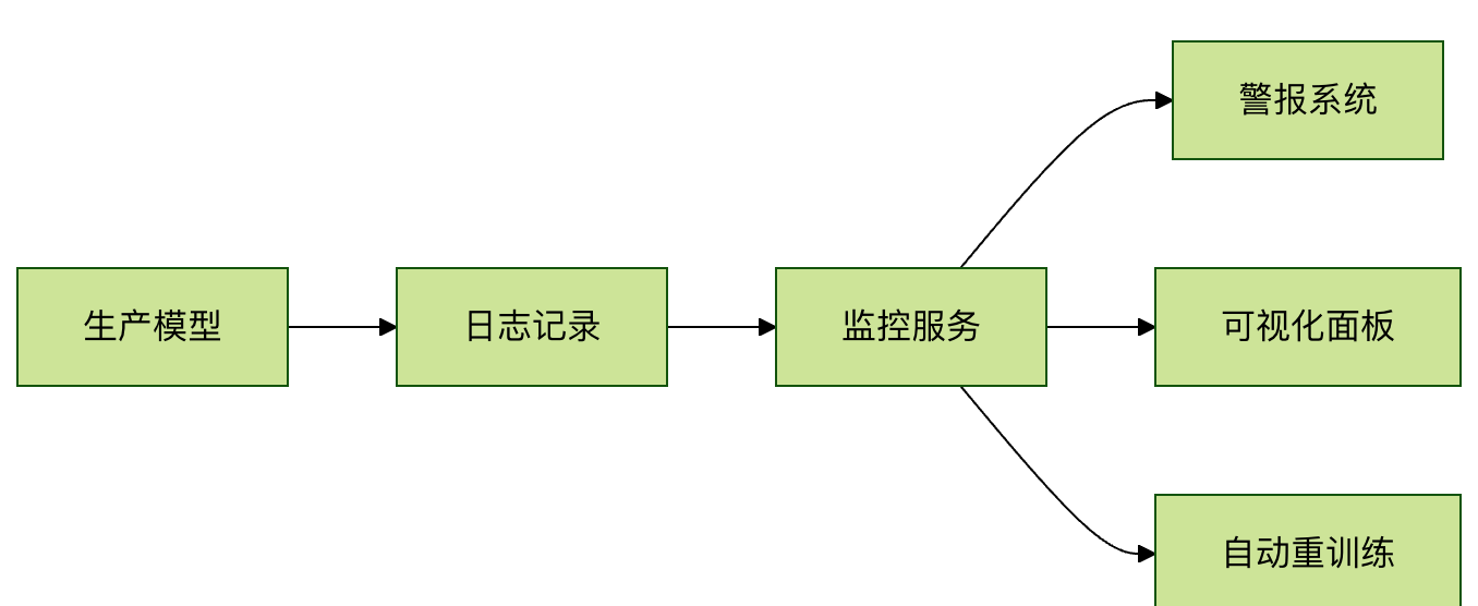
5.1 Key Points for Production Environment Monitoring
- Data drift detection: Monitor changes in input data distribution
- Concept drift detection: Monitor changes in the relationship between features and targets
- Performance degradation detection: Periodically evaluate model performance
- Anomalous input detection: Identify anomalous input samples
5.2 Monitoring System Architecture
6. Hands-On Practice
6.1 Practice Tasks
- Train a simple CNN model on the MNIST dataset
- Implement the following evaluation features:
- Accuracy and loss monitoring during the training process
- Confusion matrix analysis on the test set
- Use TensorBoard to visualize the training process
- Try to implement custom evaluation metrics
6.2 Reference Code Framework
Example
import tensorflow as tf
from tensorflow.keras import layers
# 1. Data preparation
(train_images, train_labels), (test_images, test_labels) = tf.keras.datasets.mnist.load_data()
train_images = train_images.reshape((60000, 28, 28, 1)).astype('float32') / 255
test_images = test_images.reshape((10000, 28, 28, 1)).astype('float32') / 255
# 2. Model construction
model = tf.keras.Sequential([
layers.Conv2D(32, (3, 3), activation='relu', input_shape=(28, 28, 1)),
layers.MaxPooling2D((2, 2)),
layers.Flatten(),
layers.Dense(10, activation='softmax')
])
# 3. Compile the model (add the metrics you choose)
model.compile(...)
# 4. Train the model (add TensorBoard callback)
history = model.fit(...)
# 5. Evaluate the model
test_loss, test_acc = model.evaluate(...)
# 6. Confusion matrix analysis
# Your code...
from tensorflow.keras import layers
# 1. Data preparation
(train_images, train_labels), (test_images, test_labels) = tf.keras.datasets.mnist.load_data()
train_images = train_images.reshape((60000, 28, 28, 1)).astype('float32') / 255
test_images = test_images.reshape((10000, 28, 28, 1)).astype('float32') / 255
# 2. Model construction
model = tf.keras.Sequential([
layers.Conv2D(32, (3, 3), activation='relu', input_shape=(28, 28, 1)),
layers.MaxPooling2D((2, 2)),
layers.Flatten(),
layers.Dense(10, activation='softmax')
])
# 3. Compile the model (add the metrics you choose)
model.compile(...)
# 4. Train the model (add TensorBoard callback)
history = model.fit(...)
# 5. Evaluate the model
test_loss, test_acc = model.evaluate(...)
# 6. Confusion matrix analysis
# Your code...