R Data Types
Data types refer to a broad system used to declare variables or functions of different types.
The type of a variable determines the space it occupies in storage, and how the stored bit pattern is interpreted.
There are mainly three most basic data types in R language:
- Numeric
- Logical
- Text
There are mainly two types of numeric constants:
| General type | 123 -0.125 |
|---|---|
| Scientific notation | 1.23e2 -1.25E-1 |
Logical type is often called Boolean in many other programming languages, and its constant values are onlyTRUEandFALSE。
Note:R language is case-sensitive; true or True cannot represent TRUE.
The most intuitive data type is the text type. Text is the string (String) often seen in other languages, and constants are enclosed in double quotes. In R, text constants can be enclosed in either single quotes or double quotes, for example:
Example
[1] TRUE
Regarding variable definition in R, unlike the syntax rules in some strongly typed languages where you need to specifically set a name and data type for a variable, whenever you use an assignment operator in R, you are actually defining a new variable:
Example
b <- TRUE
b = "abc"
Divided by object type, there are the following 6 types (these will be introduced in detail later):
- Vector
- List
- Matrix
- Array
- Factor
- Data frame
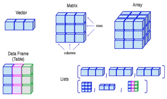
Vector
Vector is often provided in the standard libraries of specialized programming languages such as Java, Rust, and C#, because vector is an indispensable tool in mathematical operations — the most common vector we encounter is the two-dimensional vector, which is necessarily used in a plane coordinate system.
From a data structure perspective, a vector is a linear list, which can be viewed as an array.
In R, the existence of vector as a type makes vector operations easier:
Example
> b = c(5, 0)
> a + b
[1] 8 4
>
c()is a function that creates vectors.
Here two two-dimensional vectors are added to get a new two-dimensional vector (8, 4). If you perform an operation on a two-dimensional vector and a three-dimensional vector, it will lose mathematical meaning; although it will not stop running, a warning will be issued.
I suggest everyone get into the habit of preventing this situation from occurring.
Each element in a vector can be extracted individually by index:
Example
> a[2]
[1] 20
Note:In R, the "index" does not represent an offset, but represents the ordinal position, that is, it starts from 1!
R can also easily extract a portion of a vector:
Example
[1] 10 20 30 40
> a[c(1, 3, 5)] # Extract items 1, 3, 5
[1] 10 30 50
> a[c(-1, -5)] # Remove items 1 and 5
[1] 20 30 40
These three partial extraction methods are the most commonly used.
Vectors support scalar calculations:
Example
[1] 0.6 0.7 0.8
> a = c(1,2)
> a ^ 2
[1] 1 4
The commonly used mathematical functions described earlier, such as sqrt, exp, etc., can also be used for scalar operations on vectors.
As a linear list structure, "vector" should have some common linear list processing functions; R does have these functions:
Vector sorting:
Example
> sort(a)
[1] 1 2 3 4 5 6
> rev(a)
[1] 6 4 2 5 3 1
> order(a)
[1] 1 4 2 5 3 6
> a[order(a)]
[1] 1 2 3 4 5 6
The order() function returns an index vector after sorting the vector.
Vector statistics
R has very complete statistical functions:
| Function name | Meaning |
|---|---|
| sum | Sum |
| mean | Average |
| var | Variance |
| sd | Standard deviation |
| min | Minimum value |
| max | Maximum value |
| range | Range (maximum and minimum values) |
Vector statistics example:
Example
[1] 15
> sd(1:5)
[1] 1.581139
> range(1:5)
[1] 1 5
Vector generation
Vectors can be generated usingc()function, or use the min:max operator to generate a continuous sequence.
If you want to generate an arithmetic sequence with intervals, you can use the seq function:
> seq(1, 9, 2)
[1] 1 3 5 7 9
seq can also generate an arithmetic sequence from m to n, just specify m, n and the length of the sequence:
> seq(0, 1, length.out=3)
[1] 0.0 0.5 1.0
rep means repeat, and can be used to generate repeated number sequences:
> rep(0, 5)
[1] 0 0 0 0 0
NA and NULL are often used in vectors. Here we introduce these two terms and their differences:
- NA represents "missing", NULL represents "non-existent".
- NA missing is like a placeholder, meaning there is no value here, but the position exists.
- NULL means the data does not exist.
Example explanation:
Example
[1] 2
> c(NA, NA, NULL, NA)
[1] NA NA NA
Obviously, NULL has no meaning in a vector.
Logical
Logical vectors are mainly used for logical operations on vectors, for example:
Example
[1] FALSE FALSE TRUE
The which function is a very common logical vector processing function, which can be used to filter the indices of the data we need:
Example
> b = a > 12
> print(b)
[1] FALSE FALSE TRUE
> which(b)
[1] 3
For example, we need to filter data greater than or equal to 60 and less than 70 from a linear list:
Example
> print(vector[which(vector >= 60 & vector < 70)])
[1] 64 62 69
Similar functions include all and any:
Example
[1] TRUE
> all(c(TRUE, TRUE, FALSE))
[1] FALSE
> any(c(TRUE, FALSE, FALSE))
[1] TRUE
> any(c(FALSE, FALSE, FALSE))
[1] FALSE
all() is used to check whether a logical vector is all TRUE, any() is used to check whether a logical vector contains TRUE.
String
The string data type itself is not complicated; here we focus on introducing string operation functions:
Example
[1] "EXAMPLE"
> tolower("Example") # Convert to lowercase
[1] "example"
> nchar(Chinese, type="bytes") # Count byte length
[1] 4
> nchar(Chinese, type="char") # Count number of characters
[1] 2
> substr("123456789", 1, 5) # Extract substring, from 1 to 5
[1] "12345"
> substring("1234567890", 5) # Extract substring, from 5 to end
[1] "567890"
> as.numeric("12") # Convert string to number
[1] 12
> as.character(12.34) # Convert number to string
[1] "12.34"
> strsplit("2019;10;1", ";") # Split string by delimiter
[[1]]
[1] "2019" "10" "1"
> gsub("/", "-", "2019/10/1") # Replace string
[1] "2019-10-1"
On Windows computers, the GBK encoding standard is used, so one Chinese character is two bytes. If running on a computer with UTF-8 encoding, the byte length of a single Chinese character should be 3.
R supports regular expressions in Perl language format:
Example
[1] "$ $"
For more string content, refer to:R Language String Introduction。
Matrix
R language provides a matrix type for linear algebra research. This data structure is very similar to two-dimensional arrays in other languages, but R provides language-level support for matrix operations.
First, let's look at matrix generation:
Example
> matrix(vector, 2, 3)
[,1] [,2] [,3]
[1,] 1 3 5
[2,] 2 4 6
The matrix initialization content is passed by a vector, and secondly it needs to express how many rows and columns the matrix has.
Values in the vector fill the matrix column by column. If you want to fill by row, you need to specify the byrow attribute:
Example
[,1] [,2] [,3]
[1,] 1 2 3
[2,] 4 5 6
Every value in the matrix can be directly accessed:
Example
> m1[1,1] # Row 1, Column 1
[1] 1
> m1[1,3] # Row 1, Column 3
[1] 3
In R, each column and each row of a matrix can be given a name; this process is done in batch through a string vector:
Example
> rownames(m1) = c("a", "b")
> m1
x y z
a 1 2 3
b 4 5 6
> m1["a", ]
x y z
1 2 3
The four basic arithmetic operations on matrices are basically the same as those on vectors; they can be performed with scalars, or with matrices of the same size at corresponding positions.
Matrix multiplication:
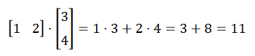
Example
> m2 = matrix(c(3, 4), 2, 1)
> m1 %*% m2
[,1]
[1,] 11
Inverse matrix:
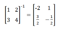
Example
> solve(A)
[,1] [,2]
[1,] -2.0 1.0
[2,] 1.5 -0.5
solve()function is used to solve linear algebra equations; the basic usage issolve(A,b), where,Ais the coefficient matrix of the equation system,bthe vector or matrix in the equation.
apply()function can treat each row or column of a matrix as a vector for operations:
Example
[,1] [,2]
[1,] 1 2
[2,] 3 4
> apply(A, 1, sum) # The second parameter is 1 for row-wise operation, use the sum() function
[1] 3 7
> apply(A, 2, sum) # The second parameter is 2 for column-wise operation
[1] 4 6
For more matrix content, refer to:R Matrix。
Other extensions