PyTorch Convolutional Neural Network
PyTorch Convolutional Neural Network (CNN) is a class of deep learning models specifically designed to process data with a grid-like topology (such as images).
CNN is a core technology for computer vision tasks (such as image classification, object detection, and segmentation).
The following diagram shows the structure and workflow of a typical Convolutional Neural Network (CNN) used for image recognition tasks.
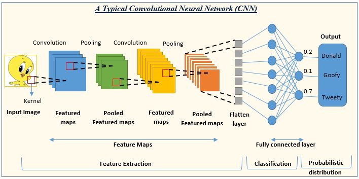
In the figure, the CNN output layer gives probabilities for three classes: Donald (0.2), Goofy (0.1), and Tweety (0.7), indicating that the network believes the input image is most likely Tweety.
The following is a brief description of each part:
-
Input Image: The raw image data received by the network.
-
Convolution: A kernel slides over the input image to extract features and generate feature maps.
-
Pooling: Usually applied after the convolutional layer, max pooling or average pooling reduces the size of feature maps while preserving important features, producing pooled feature maps.
-
Feature Extraction: The combination of multiple convolutional and pooling layers gradually extracts high-level features from the image.
-
Flatten Layer: Converts the multi-dimensional feature maps into a one-dimensional vector for input into the fully connected layer.
-
Fully Connected Layer: Similar to traditional neural network layers, it maps the extracted features to output classes.
-
Classification: The output layer of the network performs classification based on the output of the fully connected layer.
-
Probabilistic Distribution: The output layer gives the probability for each class, representing the likelihood that the input image belongs to each class.
Basic Structure of Convolutional Neural Networks
1. Input Layer
It receives the raw image data. An image is typically represented as a three-dimensional array, where two dimensions represent the width and height of the image, and the third dimension represents the color channels (for example, an RGB image has three channels).
2. Convolutional Layer
It uses convolution kernels to extract local features, such as edges and textures.
Formula:

- x: input image.
- k: convolution kernel (weight matrix).
- b: bias.
A group of learnable filters (or convolution kernels) is applied to the input image via convolution operations to extract local features.
Each filter slides over the input image and generates a feature map, representing the filter's activation at different positions.
A convolutional layer can have multiple filters; each filter generates a feature map, and all feature maps form a set of feature maps.
3. Activation Function
A nonlinear activation function, such as ReLU (Rectified Linear Unit), is usually applied after the convolutional layer to introduce nonlinearity, enabling the network to learn more complex patterns.
The ReLU function is defined as:f(x)=max(0,x), that is, if the input is less than 0, output 0; otherwise, output the input value.
4. Pooling Layer
- It is used to reduce the spatial dimensions of feature maps, decreasing the computational cost and number of parameters while retaining the most important feature information.
- The most common pooling operations are max pooling and average pooling.
- Max pooling selects the maximum value in the region, while average pooling computes the average value in the region.
5. Normalization Layer (optional)
- For example, Local Response Normalization (LRN) or Batch Normalization.
- These layers help accelerate the training process and improve model stability.
6. Fully Connected Layer
- At the end of a CNN, the feature maps extracted by earlier layers are flattened into a one-dimensional vector and then fed into the fully connected layer.
- Every neuron in the fully connected layer is connected to all neurons in the previous layer, combining features for the final classification or regression.
7. Output Layer
Depending on the task, the output layer can take different forms.
For classification tasks, the Softmax function is typically used to convert the output into a probability distribution, representing the probability of the input belonging to each class.
8. Loss Function
It is used to measure the difference between the model's predictions and the true labels.
Common loss functions include cross-entropy loss for multi-class classification tasks and mean squared error (MSE) for regression tasks.
9. Optimizer
It is used to update the network's weights based on the gradient of the loss function. Common optimizers include stochastic gradient descent (SGD), Adam, RMSprop, etc.
10. Regularization (optional)
It includes techniques such as Dropout and L1/L2 regularization to prevent the model from overfitting.
These layers can be stacked to form deeper network structures to improve the model's learning capability.
The depth and complexity of a CNN can be adjusted according to the requirements of the task.
PyTorch Implementation of a CNN Example
The following example shows how to build a simple CNN model with PyTorch for digit classification on the MNIST dataset.
Main Steps:
- Data Loading and Preprocessing: Use
torchvisionload and preprocess the MNIST data. - Model Construction: Define convolutional, pooling, and fully connected layers.
- Training: Train the model using a loss function and an optimizer.
- Evaluation: Calculate the model's accuracy on the test set.
- Visualization: Display some test samples and their prediction results.
1. Import Required Libraries
import torch
import torch.nn as nn
import torch.nn.functional as F
import torch.optim as optim
2. Data Loading
Use the MNIST dataset provided by torchvision to load and preprocess the data.
Example
transforms.ToTensor(), # Convert to tensor
transforms.Normalize((0.5,), (0.5,)) # Normalize to [-1, 1]
])
# Load MNIST dataset
train_dataset = datasets.MNIST(root='./data', train=True, transform=transform, download=True)
test_dataset = datasets.MNIST(root='./data', train=False, transform=transform, download=True)
train_loader = torch.utils.data.DataLoader(dataset=train_dataset, batch_size=64, shuffle=True)
test_loader = torch.utils.data.DataLoader(dataset=test_dataset, batch_size=64, shuffle=False)
3. Define the CNN Model
Usenn.Modulebuild a CNN.Example
def __init__(self):
super(SimpleCNN, self).__init__()
# Define convolutional layer: 1 input channel, 32 output channels, kernel size 3x3
self.conv1 = nn.Conv2d(1, 32, kernel_size=3, stride=1, padding=1)
# Define convolutional layer: 32 input channels, 64 output channels
self.conv2 = nn.Conv2d(32, 64, kernel_size=3, stride=1, padding=1)
# Define fully connected layer
self.fc1 = nn.Linear(64 * 7 * 7, 128) # Input size = feature map size * number of channels
self.fc2 = nn.Linear(128, 10) # 10 classes
def forward(self, x):
x = F.relu(self.conv1(x)) # First convolutional layer + ReLU
x = F.max_pool2d(x, 2) # Max pooling
x = F.relu(self.conv2(x)) # Second convolutional layer + ReLU
x = F.max_pool2d(x, 2) # Max pooling
x = x.view(-1, 64 * 7 * 7) # Flatten operation
x = F.relu(self.fc1(x)) # Fully connected layer + ReLU
x = self.fc2(x) # Fully connected layer output
return x
# Create model instance
model = SimpleCNN()
4. Define Loss Function and Optimizer
Use cross-entropy loss and stochastic gradient descent optimizer.
criterion = nn.CrossEntropyLoss()  # 多分类交叉熵损失
optimizer = optim.SGD(model.parameters(), lr=0.01, momentum=0.9)  # 学习率和动量
5. Train the Model
Train the model for 5 epochs, and output the training loss after each epoch.
Example
model.train() # Set to training mode
for epoch in range(num_epochs):
total_loss = 0
for images, labels in train_loader:
# Forward pass
outputs = model(images)
loss = criterion(outputs, labels)
# Backward pass
optimizer.zero_grad()
loss.backward()
optimizer.step()
total_loss += loss.item()
print(f"Epoch [{epoch+1}/{num_epochs}], Loss: {total_loss / len(train_loader):.4f}")
6. Test the Model
Evaluate the model's accuracy on the test set.
Example
correct = 0
total = 0
with torch.no_grad(): # No gradient calculation needed during evaluation
for images, labels in test_loader:
outputs = model(images)
_, predicted = torch.max(outputs, 1) # Predict classes
total += labels.size(0)
correct += (predicted == labels).sum().item()
accuracy = 100 * correct / total
print(f"Test Accuracy: {accuracy:.2f}%")
7. Complete Code
The complete code is as follows:
Example
import torch.nn as nn
import torch.nn.functional as F
import torch.optim as optim
from torchvision import datasets, transforms
# 1. Data loading and preprocessing
transform = transforms.Compose([
transforms.ToTensor(), # Convert to tensor
transforms.Normalize((0.5,), (0.5,)) # Normalize to [-1, 1]
])
# Load MNIST dataset
train_dataset = datasets.MNIST(root='./data', train=True, transform=transform, download=True)
test_dataset = datasets.MNIST(root='./data', train=False, transform=transform, download=True)
train_loader = torch.utils.data.DataLoader(dataset=train_dataset, batch_size=64, shuffle=True)
test_loader = torch.utils.data.DataLoader(dataset=test_dataset, batch_size=64, shuffle=False)
# 2. Define CNN model
class SimpleCNN(nn.Module):
def __init__(self):
super(SimpleCNN, self).__init__()
# Define convolutional layers
self.conv1 = nn.Conv2d(1, 32, kernel_size=3, stride=1, padding=1) # Input 1 channel, output 32 channels
self.conv2 = nn.Conv2d(32, 64, kernel_size=3, stride=1, padding=1) # Input 32 channels, output 64 channels
# Define fully connected layers
self.fc1 = nn.Linear(64 * 7 * 7, 128) # Flatten and feed into fully connected layer
self.fc2 = nn.Linear(128, 10) # 10 classes
def forward(self, x):
x = F.relu(self.conv1(x)) # First convolution + ReLU
x = F.max_pool2d(x, 2) # Max pooling
x = F.relu(self.conv2(x)) # Second convolution + ReLU
x = F.max_pool2d(x, 2) # Max pooling
x = x.view(-1, 64 * 7 * 7) # Flatten
x = F.relu(self.fc1(x)) # Fully connected layer + ReLU
x = self.fc2(x) # Final output layer
return x
# Create model instance
model = SimpleCNN()
# 3. Define loss function and optimizer
criterion = nn.CrossEntropyLoss() # Multi-class cross-entropy loss
optimizer = optim.SGD(model.parameters(), lr=0.01, momentum=0.9)
# 4. Model training
num_epochs = 5
model.train() # Set model to training mode
for epoch in range(num_epochs):
total_loss = 0
for images, labels in train_loader:
outputs = model(images) # Forward pass
loss = criterion(outputs, labels) # Compute loss
optimizer.zero_grad() # Clear gradients
loss.backward() # Backward pass
optimizer.step() # Update parameters
total_loss += loss.item()
print(f"Epoch [{epoch+1}/{num_epochs}], Loss: {total_loss / len(train_loader):.4f}")
# 5. Model testing
model.eval() # Set model to evaluation mode
correct = 0
total = 0
with torch.no_grad(): # Disable gradient computation
for images, labels in test_loader:
outputs = model(images)
_, predicted = torch.max(outputs, 1)
total += labels.size(0)
correct += (predicted == labels).sum().item()
accuracy = 100 * correct / total
print(f"Test Accuracy: {accuracy:.2f}%")
Explanation of Running Results
1. Output training loss
The code outputs an average loss after each epoch, for example:
Epoch [1/5], Loss: 0.2325
Epoch [2/5], Loss: 0.0526
Epoch [3/5], Loss: 0.0366
Epoch [4/5], Loss: 0.0273
Epoch [5/5], Loss: 0.0221
Explanation:The gradual decrease in loss indicates that the model is converging step by step.
2. Accuracy on the test set
The code outputs the final classification accuracy on the test set, for example:
Test Accuracy: 98.96%
Explanation:The model achieves a classification accuracy of 98.96% on the MNIST test set, which is a good result for a simple CNN model.
7. Visualize Results
We can visualize some samples and their prediction results in the test data.
Example
import torch.nn as nn
import torch.nn.functional as F
import torch.optim as optim
from torchvision import datasets, transforms
import matplotlib.pyplot as plt
# 1. Data loading and preprocessing
transform = transforms.Compose([
transforms.ToTensor(), # Convert to tensor
transforms.Normalize((0.5,), (0.5,)) # Normalize to [-1, 1]
])
# Load MNIST dataset
train_dataset = datasets.MNIST(root='./data', train=True, transform=transform, download=True)
test_dataset = datasets.MNIST(root='./data', train=False, transform=transform, download=True)
train_loader = torch.utils.data.DataLoader(dataset=train_dataset, batch_size=64, shuffle=True)
test_loader = torch.utils.data.DataLoader(dataset=test_dataset, batch_size=64, shuffle=False)
# 2. Define CNN model
class SimpleCNN(nn.Module):
def __init__(self):
super(SimpleCNN, self).__init__()
# Define convolutional layers
self.conv1 = nn.Conv2d(1, 32, kernel_size=3, stride=1, padding=1) # Input 1 channel, output 32 channels
self.conv2 = nn.Conv2d(32, 64, kernel_size=3, stride=1, padding=1) # Input 32 channels, output 64 channels
# Define fully connected layers
self.fc1 = nn.Linear(64 * 7 * 7, 128) # Flatten and feed into fully connected layer
self.fc2 = nn.Linear(128, 10) # 10 classes
def forward(self, x):
x = F.relu(self.conv1(x)) # First convolution + ReLU
x = F.max_pool2d(x, 2) # Max pooling
x = F.relu(self.conv2(x)) # Second convolution + ReLU
x = F.max_pool2d(x, 2) # Max pooling
x = x.view(-1, 64 * 7 * 7) # Flatten
x = F.relu(self.fc1(x)) # Fully connected layer + ReLU
x = self.fc2(x) # Final output layer
return x
# Create model instance
model = SimpleCNN()
# 3. Define loss function and optimizer
criterion = nn.CrossEntropyLoss() # Multi-class cross-entropy loss
optimizer = optim.SGD(model.parameters(), lr=0.01, momentum=0.9)
# 4. Model training
num_epochs = 5
model.train() # Set model to training mode
for epoch in range(num_epochs):
total_loss = 0
for images, labels in train_loader:
outputs = model(images) # Forward pass
loss = criterion(outputs, labels) # Compute loss
optimizer.zero_grad() # Clear gradients
loss.backward() # Backward pass
optimizer.step() # Update parameters
total_loss += loss.item()
print(f"Epoch [{epoch+1}/{num_epochs}], Loss: {total_loss / len(train_loader):.4f}")
# 5. Model testing
model.eval() # Set model to evaluation mode
correct = 0
total = 0
with torch.no_grad(): # Disable gradient computation
for images, labels in test_loader:
outputs = model(images)
_, predicted = torch.max(outputs, 1)
total += labels.size(0)
correct += (predicted == labels).sum().item()
accuracy = 100 * correct / total
print(f"Test Accuracy: {accuracy:.2f}%")
# 6. Visualize test results
dataiter = iter(test_loader)
images, labels = next(dataiter)
outputs = model(images)
_, predictions = torch.max(outputs, 1)
fig, axes = plt.subplots(1, 6, figsize=(12, 4))
for i in range(6):
axes[i].imshow(images[i][0], cmap='gray')
axes[i].set_title(f"Label: {labels[i]}\nPred: {predictions[i]}")
axes[i].axis('off')
plt.show()
The visualization results show the actual labels and predicted values of 6 test samples, for example:
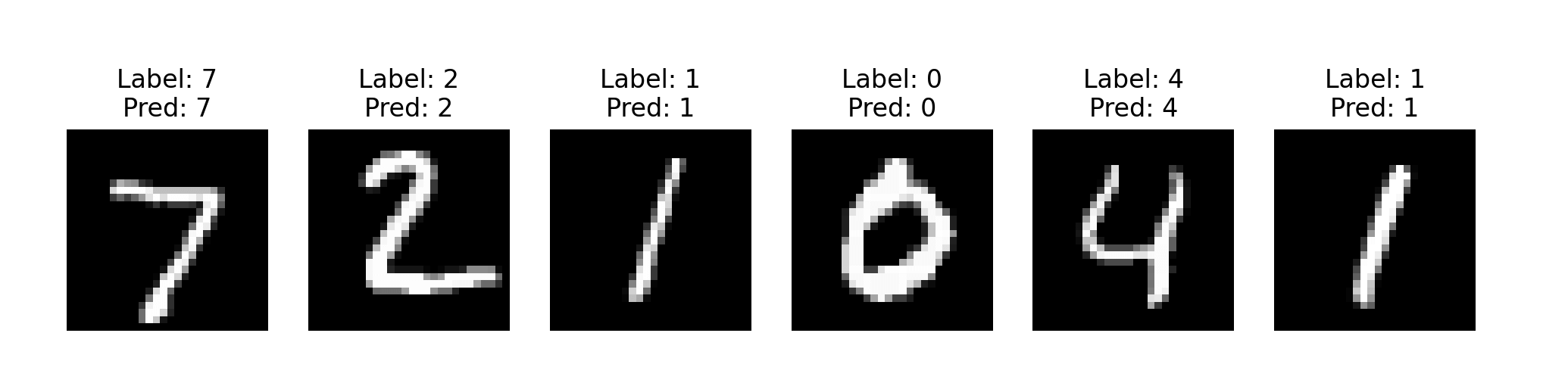
The upper left corner of the image is the handwritten digit.
The title section shows the model's predicted value and the true label.
Note Several Common Errors
When downloading the MNIST dataset, the download fails due to SSL certificate verification failure.
Downloading http://yann.lecun.com/exdb/mnist/train-images-idx3-ubyte.gz
Failed to download (trying next):
<urlopen error [SSL: CERTIFICATE_VERIFY_FAILED] certificate verify failed: unable to get local issuer certificate (_ssl.c:1129)>
...
Solutions
Open a terminal and run the following command to install/update the SSL certificate:
/Applications/Python\ 3.x/Install\ Certificates.command
Replace 3.x with the Python version you actually installed.
After running this command, re-run your Python code and it should be able to download the MNIST dataset successfully.
Other extensions