PyTorch First Neural Network
In this chapter, we will introduce how to use PyTorch to implement a simple feedforward neural network to complete a binary classification task.
The following example demonstrates how to use PyTorch to implement a simple neural network for binary classification training.
The network structure includes an input layer, a hidden layer, and an output layer, using ReLU activation function and Sigmoid activation function.
It uses mean squared error loss function and stochastic gradient descent optimizer.
The training process gradually adjusts model parameters through forward propagation, loss calculation, backward propagation, and parameter updates.
Example
import torch
import torch.nn as nn
# Define input layer size, hidden layer size, output layer size, and batch size
n_in, n_h, n_out, batch_size = 10, 5, 1, 10
# Create dummy input data and target data
x = torch.randn(batch_size, n_in) # Randomly generate input data
y = torch.tensor([[1.0], [0.0], [0.0],
[1.0], [1.0], [1.0], [0.0], [0.0], [1.0], [1.0]]) # Target output data
# Create a sequential model with linear layers, ReLU activation function, and Sigmoid activation function
model = nn.Sequential(
nn.Linear(n_in, n_h), # Linear transformation from input layer to hidden layer
nn.ReLU(), # ReLU activation function for hidden layer
nn.Linear(n_h, n_out), # Linear transformation from hidden layer to output layer
nn.Sigmoid() # Sigmoid activation function for output layer
)
# Define mean squared error loss function and stochastic gradient descent optimizer
criterion = torch.nn.MSELoss()
optimizer = torch.optim.SGD(model.parameters(), lr=0.01) # Learning rate is 0.01
# Execute gradient descent algorithm for model training
for epoch in range(50): # Iterate 50 times
y_pred = model(x) # Forward propagation, compute predicted values
loss = criterion(y_pred, y) # Compute loss
print('epoch: ', epoch, 'loss: ', loss.item()) # Print loss value
optimizer.zero_grad() # Clear gradients
loss.backward() # Backward propagation, compute gradients
optimizer.step() # Update model parameters
The output result is similar to the following:
epoch:  0 loss:  0.2591968774795532
epoch:  1 loss:  0.25902628898620605
epoch:  2 loss:  0.25885599851608276
epoch:  3 loss:  0.25868603587150574
epoch:  4 loss:  0.25851646065711975
...
Define network parameters:
n_in, n_h, n_out, batch_size = 10, 5, 1, 10
n_in: The input layer size is 10, meaning each data point has 10 features.n_h: The hidden layer size is 5, meaning the hidden layer contains 5 neurons.n_out: The output layer size is 1, i.e., it outputs a scalar representing the binary classification result (0 or 1).batch_size: Each batch contains 10 samples.
Generate input data and target data:
x = torch.randn(batch_size, n_in)  # 随机生成输入数据
y = torch.tensor([[1.0], [0.0], [0.0],
                 [1.0], [1.0], [1.0], [0.0], [0.0], [1.0], [1.0]])  # 目标输出数据
x: Randomly generate a shape of(10, 10)input data matrix, representing 10 samples, each sample has 10 features.y: Target output data (labels), representing the class label (0 or 1) for each input sample, is a 10×1 tensor.
Define the neural network model:
model = nn.Sequential(
   nn.Linear(n_in, n_h),  # 输入层到隐藏层的线性变换
   nn.ReLU(),            # 隐藏层的ReLU激活函数
   nn.Linear(n_h, n_out),  # 隐藏层到输出层的线性变换
   nn.Sigmoid()           # 输出层的Sigmoid激活函数
)
nn.SequentialUsed to define network layers in sequence.
nn.Linear(n_in, n_h): Defines the linear transformation from input layer to hidden layer, with 10 input features and 5 neurons in the hidden layer.nn.ReLU(): Adds ReLU activation function after the hidden layer to increase non-linearity.nn.Linear(n_h, n_out): Defines the linear transformation from hidden layer to output layer, with 1 output neuron.nn.Sigmoid(): The output layer uses Sigmoid activation function to map the result to between 0 and 1 for binary classification.
Define loss function and optimizer:
criterion = torch.nn.MSELoss()  # 使用均方误差损失函数
optimizer = torch.optim.SGD(model.parameters(), lr=0.01)  # 使用随机梯度下降优化器,学习率为 0.01
Training loop:
for epoch in range(50):  # 训练50轮
   y_pred = model(x)  # 前向传播,计算预测值
   loss = criterion(y_pred, y)  # 计算损失
   print('epoch: ', epoch, 'loss: ', loss.item())  # 打印损失值

   optimizer.zero_grad()  # 清零梯度
   loss.backward()  # 反向传播,计算梯度
   optimizer.step()  # 更新模型参数
for epoch in range(50): Perform 50 training iterations.y_pred = model(x): Perform forward propagation, using current model parameters to compute the input datax's predicted values.loss = criterion(y_pred, y): Compute the predicted values and target valuesythe loss between.optimizer.zero_grad(): Clear the gradient values from the previous training round.loss.backward(): Backward propagation, compute the gradient of the loss function with respect to the model parameters.optimizer.step(): Update the model parameters based on the computed gradients.
Visualization code:
Example
import torch.nn as nn
import matplotlib.pyplot as plt
# Define input layer size, hidden layer size, output layer size, and batch size
n_in, n_h, n_out, batch_size = 10, 5, 1, 10
# Create dummy input data and target data
x = torch.randn(batch_size, n_in) # Randomly generate input data
y = torch.tensor([[1.0], [0.0], [0.0],
[1.0], [1.0], [1.0], [0.0], [0.0], [1.0], [1.0]]) # Target output data
# Create a sequential model with linear layers, ReLU activation function, and Sigmoid activation function
model = nn.Sequential(
nn.Linear(n_in, n_h), # Linear transformation from input layer to hidden layer
nn.ReLU(), # ReLU activation function for hidden layer
nn.Linear(n_h, n_out), # Linear transformation from hidden layer to output layer
nn.Sigmoid() # Sigmoid activation function for output layer
)
# Define mean squared error loss function and stochastic gradient descent optimizer
criterion = torch.nn.MSELoss()
optimizer = torch.optim.SGD(model.parameters(), lr=0.01) # Learning rate is 0.01
# Used to store the loss value for each epoch
losses = []
# Execute gradient descent algorithm for model training
for epoch in range(50): # Iterate 50 times
y_pred = model(x) # Forward propagation, compute predicted values
loss = criterion(y_pred, y) # Compute loss
losses.append(loss.item()) # Record loss value
print(f'Epoch [{epoch+1}/50], Loss: {loss.item():.4f}') # Print loss value
optimizer.zero_grad() # Clear gradients
loss.backward() # Backward propagation, compute gradients
optimizer.step() # Update model parameters
# Visualize the loss curve
plt.figure(figsize=(8, 5))
plt.plot(range(1, 51), losses, label='Loss')
plt.xlabel('Epoch')
plt.ylabel('Loss')
plt.title('Training Loss Over Epochs')
plt.legend()
plt.grid()
plt.show()
# Visualize comparison of predicted results with actual target values
y_pred_final = model(x).detach().numpy() # Final predicted values
y_actual = y.numpy() # Actual values
plt.figure(figsize=(8, 5))
plt.plot(range(1, batch_size + 1), y_actual, 'o-', label='Actual', color='blue')
plt.plot(range(1, batch_size + 1), y_pred_final, 'x--', label='Predicted', color='red')
plt.xlabel('Sample Index')
plt.ylabel('Value')
plt.title('Actual vs Predicted Values')
plt.legend()
plt.grid()
plt.show()
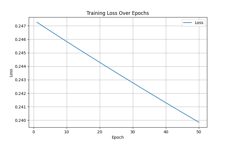
Displayed as follows:
Another Example
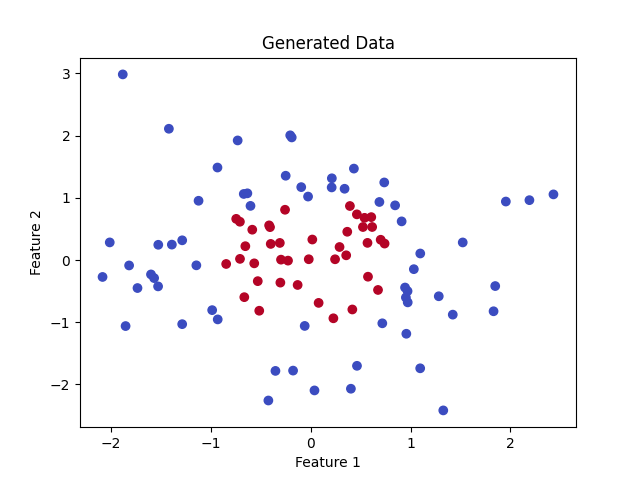
We assume there is a two-dimensional dataset, and the goal is to classify the points into two categories based on their positions (e.g., red and blue points).
The following example demonstrates how to use a neural network to complete a simple binary classification task, laying a foundation for more complex tasks. With PyTorch's modular interface, building, training, and visualizing neural networks are very intuitive.
1. Data Preparation
First, we generate some simple two-dimensional data:
Example
import torch.nn as nn
import torch.optim as optim
import matplotlib.pyplot as plt
# Generate some random data
n_samples = 100
data = torch.randn(n_samples, 2) # Generate 100 two-dimensional data points
labels = (data[:, 0]**2 + data[:, 1]**2 < 1).float().unsqueeze(1) # Point inside the circle is 1, outside the circle is 0
# Visualize data
plt.scatter(data[:, 0], data[:, 1], c=labels.squeeze(), cmap='coolwarm')
plt.title("Generated Data")
plt.xlabel("Feature 1")
plt.ylabel("Feature 2")
plt.show()
Data description:
dataIs the input two-dimensional point, each point has two features.labelsIs the target classification, 1 if the point is inside the circular region, otherwise 0.
Displayed as follows:
2. Define Neural Network
Use PyTorch to create a simple feedforward neural network.
The feedforward neural network uses one hidden layer, capturing nonlinear patterns in the data through simple linear transformations and activation functions.
Example
def __init__(self):
super(SimpleNN, self).__init__()
# Define the layers of the neural network
self.fc1 = nn.Linear(2, 4) # Input layer has 2 features, hidden layer has 4 neurons
self.fc2 = nn.Linear(4, 1) # Hidden layer outputs to 1 neuron (for binary classification)
self.sigmoid = nn.Sigmoid() # Binary classification activation function
def forward(self, x):
x = torch.relu(self.fc1(x)) # Use ReLU activation function
x = self.sigmoid(self.fc2(x)) # Output layer uses Sigmoid activation function
return x
# Instantiate the model
model = SimpleNN()
3. Define Loss Function and Optimizer
Example
criterion = nn.BCELoss() # Binary cross entropy loss
optimizer = optim.SGD(model.parameters(), lr=0.1) # Use stochastic gradient descent optimizer
4. Train Model
Train the model with data so that it learns to classify.
Example
epochs = 100
for epoch in range(epochs):
# Forward propagation
outputs = model(data)
loss = criterion(outputs, labels)
# Backward propagation
optimizer.zero_grad()
loss.backward()
optimizer.step()
# Print loss every 10 epochs
if (epoch + 1) % 10 == 0:
print(f'Epoch [{epoch + 1}/{epochs}], Loss: {loss.item():.4f}')
5. Test Model and Visualize Results
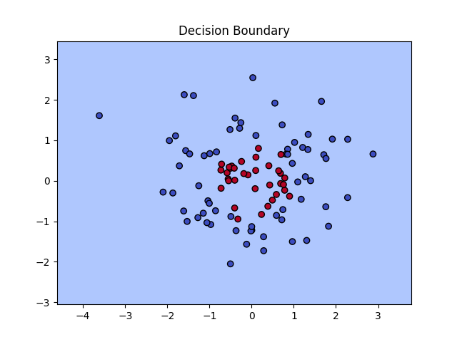
We test the model and plot the decision boundary on the image.
Example
def plot_decision_boundary(model, data):
x_min, x_max = data[:, 0].min() - 1, data[:, 0].max() + 1
y_min, y_max = data[:, 1].min() - 1, data[:, 1].max() + 1
xx, yy = torch.meshgrid(torch.arange(x_min, x_max, 0.1), torch.arange(y_min, y_max, 0.1), indexing='ij')
grid = torch.cat([xx.reshape(-1, 1), yy.reshape(-1, 1)], dim=1)
predictions = model(grid).detach().numpy().reshape(xx.shape)
plt.contourf(xx, yy, predictions, levels=[0, 0.5, 1], cmap='coolwarm', alpha=0.7)
plt.scatter(data[:, 0], data[:, 1], c=labels.squeeze(), cmap='coolwarm', edgecolors='k')
plt.title("Decision Boundary")
plt.show()
plot_decision_boundary(model, data)
6. Complete Code
The complete code is as follows:
Example
import torch.nn as nn
import torch.optim as optim
import matplotlib.pyplot as plt
# Generate some random data
n_samples = 100
data = torch.randn(n_samples, 2) # Generate 100 two-dimensional data points
labels = (data[:, 0]**2 + data[:, 1]**2 < 1).float().unsqueeze(1) # Point inside the circle is 1, outside the circle is 0
# Visualize data
plt.scatter(data[:, 0], data[:, 1], c=labels.squeeze(), cmap='coolwarm')
plt.title("Generated Data")
plt.xlabel("Feature 1")
plt.ylabel("Feature 2")
plt.show()
# Define feedforward neural network
class SimpleNN(nn.Module):
def __init__(self):
super(SimpleNN, self).__init__()
# Define the layers of the neural network
self.fc1 = nn.Linear(2, 4) # Input layer has 2 features, hidden layer has 4 neurons
self.fc2 = nn.Linear(4, 1) # Hidden layer outputs to 1 neuron (for binary classification)
self.sigmoid = nn.Sigmoid() # Binary classification activation function
def forward(self, x):
x = torch.relu(self.fc1(x)) # Use ReLU activation function
x = self.sigmoid(self.fc2(x)) # Output layer uses Sigmoid activation function
return x
# Instantiate the model
model = SimpleNN()
# Define loss function and optimizer
criterion = nn.BCELoss() # Binary cross entropy loss
optimizer = optim.SGD(model.parameters(), lr=0.1) # Use stochastic gradient descent optimizer
# Train
epochs = 100
for epoch in range(epochs):
# Forward Propagation
outputs = model(data)
loss = criterion(outputs, labels)
# Backward Propagation
optimizer.zero_grad()
loss.backward()
optimizer.step()
# Print loss every 10 epochs
if (epoch + 1) % 10 == 0:
print(f'Epoch [{epoch + 1}/{epochs}], Loss: {loss.item():.4f}')
# Visualize decision boundary
def plot_decision_boundary(model, data):
x_min, x_max = data[:, 0].min() - 1, data[:, 0].max() + 1
y_min, y_max = data[:, 1].min() - 1, data[:, 1].max() + 1
xx, yy = torch.meshgrid(torch.arange(x_min, x_max, 0.1), torch.arange(y_min, y_max, 0.1), indexing='ij')
grid = torch.cat([xx.reshape(-1, 1), yy.reshape(-1, 1)], dim=1)
predictions = model(grid).detach().numpy().reshape(xx.shape)
plt.contourf(xx, yy, predictions, levels=[0, 0.5, 1], cmap='coolwarm', alpha=0.7)
plt.scatter(data[:, 0], data[:, 1], c=labels.squeeze(), cmap='coolwarm', edgecolors='k')
plt.title("Decision Boundary")
plt.show()
plot_decision_boundary(model, data)
Loss output during training:
Epoch [10/100], Loss: 0.5247
Epoch [20/100], Loss: 0.3142
...
Epoch [100/100], Loss: 0.0957
The figure shows the original data points (red and blue), as well as the classification boundary learned by the model.