Pandas Stock Data Analysis
In stock data analysis, pandas is a very powerful tool that can help us process and analyze stock market data.
In this chapter, we use yfinance (Yahoo Finance library) to download historical stock data and perform various analyses, including data cleaning, visualization, calculation of technical indicators, etc.
yfinance is a Python library that can easily obtain historical and real-time data for assets such as stocks, funds, and cryptocurrencies from Yahoo Finance.
With pandas, we can store this data as a DataFrame and perform subsequent analysis.
- Data cleaning: Handle missing values, remove unnecessary columns, etc.
- Data visualization: Plot stock time series, moving averages, RSI, etc.
- Technical indicator calculation: Such as moving average (SMA), relative strength index (RSI), etc.
- Daily return and cumulative return analysis: Helps evaluate the short-term and long-term performance of a stock.
- Volatility analysis: Measures the price volatility of a stock.
For more financial libraries and quantitative analysis, you can refer to:Python Quantitative Trading
Install yfinance
First, we need to install the yfinance library as follows:
pip install yfinance --upgrade --no-cache-dir
When installing yfinance, pandas is usually installed automatically as a dependency. This means that when using yfinance, you can directly use the data structures and functions provided by pandas to process and analyze data.
Import the required libraries:
import yfinance as yf
import pandas as pd
import matplotlib.pyplot as plt
import seaborn as sns
Get Stock Data
Using the yfinance library, we can easily download stock data.
We usually use the yf.download() function to obtain historical data for a stock from Yahoo Finance.
Moutai's stock code is 600519.SS, where.SS.SS is the suffix for the Shanghai Stock Exchange.
Use yfinance to get stock data:
Example
# Get stock data for Moutai (600519.SS) from 2020-01-01 to 2021-01-01
stock_data = yf.download('600519.SS', start='2020-01-01', end='2021-01-01')
# View the first few rows of the data
print(stock_data.head())
The output data is shown below:

The returned data contains the following columns:
Open: OpenHigh: HighLow: LowClose: CloseAdj Close: Adjusted close (taking into account dividends, stock splits, etc.)Volume: Volume
The yf.download() function returns a pandas.DataFrame containing the historical data of the specified stock:
Example
# Get data for Moutai stock (600519.SS)
stock_data = yf.download('600519.SS', start='2020-01-01', end='2021-01-01')
# Check the data type
print(type(stock_data)) # Should output <class 'pandas.core.frame.DataFrame'>
The output is:
[*********************100%%**********************]  1 of 1 completed
<class 'pandas.core.frame.DataFrame'>
Data Cleaning and Processing
When analyzing stock data, we usually need to do some data cleaning and processing.
Common steps include filling missing values, removing irrelevant columns, data type conversion, etc.
In some versions of yfinance, pandas is automatically introduced and does not need to be imported again, so when using yfinance, you can directly use the data structures and functions provided by pandas to process and analyze data.
Check for missing values and fill them:
Example
# Get stock data for Moutai (600519.SS) from 2020-01-01 to 2021-01-01
stock_data = yf.download('600519.SS', start='2020-01-01', end='2021-01-01')
# Check for missing values
print(stock_data.isnull().sum())
# Fill missing values using forward fill
stock_data.ffill(inplace=True)
# Or use backward fill
# stock_data.bfill(inplace=True)
# Check whether missing values have been handled
print(stock_data.isnull().sum())
The output result is as follows:
[*********************100%%**********************]  1 of 1 completed
Open         0
High         0
Low          0
Close        0
Adj Close    0
Volume       0
dtype: int64
Open         0
High         0
Low          0
Close        0
Adj Close    0
Volume       0
Remove irrelevant columns:
Example
# Get stock data for Moutai (600519.SS) from 2020-01-01 to 2021-01-01
stock_data = yf.download('600519.SS', start='2020-01-01', end='2021-01-01')
# Drop the 'Volume' and 'Adj Close' columns
stock_data_cleaned = stock_data.drop(columns=['Adj Close', 'Volume'])
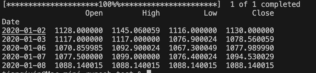
print(stock_data_cleaned.head())
The output result is as follows:
Data Visualization: Plotting Stock Price Curves
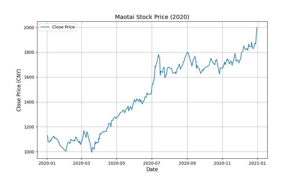
Using matplotlib or seaborn, we can visualize stock data to help us identify trends and fluctuations.
Plot the time series of the closing price:
Example
import matplotlib.pyplot as plt
# Get stock data for Moutai (600519.SS) from 2020-01-01 to 2021-01-01
stock_data = yf.download('600519.SS', start='2020-01-01', end='2021-01-01')
# Drop the 'Volume' and 'Adj Close' columns
stock_data_cleaned = stock_data.drop(columns=['Adj Close', 'Volume'])
# Plot the closing price curve of Moutai
plt.figure(figsize=(10, 6))
plt.plot(stock_data_cleaned['Close'], label='Close Price')
plt.title('Maotai Stock Price (2020)', fontsize=14)
plt.xlabel('Date', fontsize=12)
plt.ylabel('Close Price (CNY)', fontsize=12)
plt.legend()
plt.grid(True)
plt.show()
The output is as follows:
Calculating Technical Indicators for Stocks
In stock analysis, technical indicators (such as moving averages, relative strength index RSI, etc.) are often used to assist decision-making. pandas can help us calculate these indicators.
1. Moving Average (SMA)
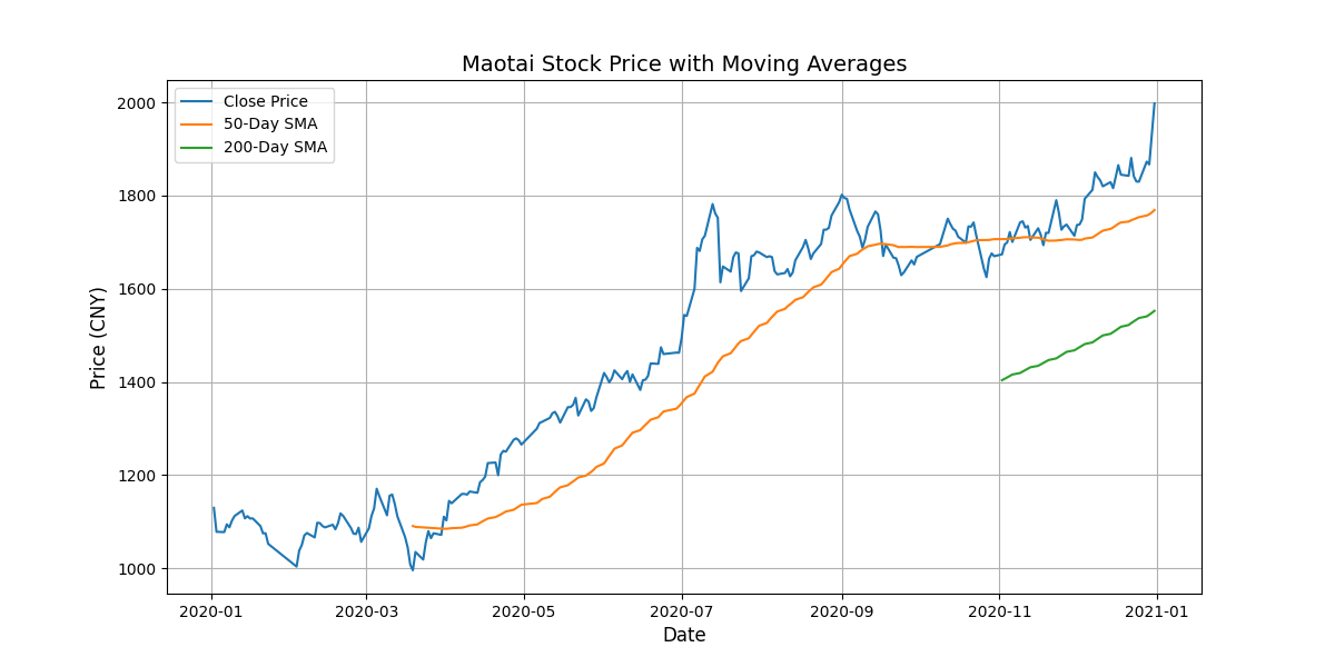
The Simple Moving Average (SMA) is one of the most commonly used technical indicators, representing the average closing price over the past N days.
Example
import matplotlib.pyplot as plt
# Get stock data for Moutai (600519.SS) from 2020-01-01 to 2021-01-01
stock_data = yf.download('600519.SS', start='2020-01-01', end='2021-01-01')
# Drop the 'Volume' and 'Adj Close' columns
stock_data_cleaned = stock_data.drop(columns=['Adj Close', 'Volume'])
# Calculate the 50-day and 200-day moving averages
stock_data_cleaned['SMA_50'] = stock_data_cleaned['Close'].rolling(window=50).mean()
stock_data_cleaned['SMA_200'] = stock_data_cleaned['Close'].rolling(window=200).mean()
# Plot the closing price and moving averages
plt.figure(figsize=(12, 6))
plt.plot(stock_data_cleaned['Close'], label='Close Price')
plt.plot(stock_data_cleaned['SMA_50'], label='50-Day SMA')
plt.plot(stock_data_cleaned['SMA_200'], label='200-Day SMA')
plt.title('Maotai Stock Price with Moving Averages', fontsize=14)
plt.xlabel('Date', fontsize=12)
plt.ylabel('Price (CNY)', fontsize=12)
plt.legend()
plt.grid(True)
plt.show()
The output is as follows:
2. Relative Strength Index (RSI)
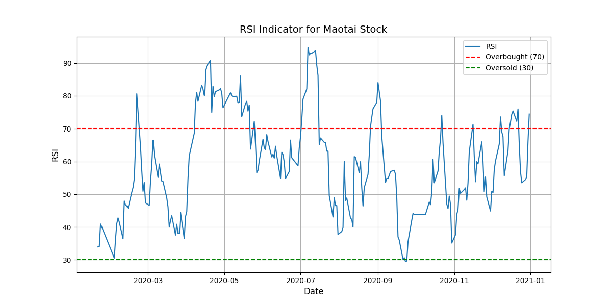
RSI is a technical indicator used to assess whether a stock is overbought or oversold. Generally speaking, an RSI greater than 70 indicates overbought, and less than 30 indicates oversold.
Example
import matplotlib.pyplot as plt
# Get stock data for Moutai (600519.SS) from 2020-01-01 to 2021-01-01
stock_data = yf.download('600519.SS', start='2020-01-01', end='2021-01-01')
# Drop the 'Volume' and 'Adj Close' columns
stock_data_cleaned = stock_data.drop(columns=['Adj Close', 'Volume'])
# Calculate the RSI indicator
delta = stock_data_cleaned['Close'].diff(1)
gain = delta.where(delta > 0, 0)
loss = -delta.where(delta < 0, 0)
# Calculate average gains and losses
avg_gain = gain.rolling(window=14).mean()
avg_loss = loss.rolling(window=14).mean()
# Calculate the Relative Strength Index (RSI)
rs = avg_gain / avg_loss
rsi = 100 - (100 / (1 + rs))
# Add RSI to the data
stock_data_cleaned['RSI'] = rsi
# Plot the RSI curve
plt.figure(figsize=(12, 6))
plt.plot(stock_data_cleaned['RSI'], label='RSI')
plt.axhline(y=70, color='r', linestyle='--', label='Overbought (70)')
plt.axhline(y=30, color='g', linestyle='--', label='Oversold (30)')
plt.title('RSI Indicator for Maotai Stock', fontsize=14)
plt.xlabel('Date', fontsize=12)
plt.ylabel('RSI', fontsize=12)
plt.legend()
plt.grid(True)
plt.show()
The output is as follows:
Applications of Stock Data Analysis
In actual stock data analysis, you can use pandas to perform the following common operations:
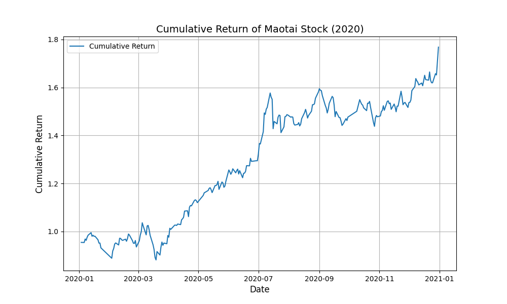
1. Daily Return and Cumulative Return
Calculating the daily return and cumulative return of a stock helps evaluate its long-term performance.
Example
import matplotlib.pyplot as plt
# Get stock data for Moutai (600519.SS) from 2020-01-01 to 2021-01-01
stock_data = yf.download('600519.SS', start='2020-01-01', end='2021-01-01')
# Drop the 'Volume' and 'Adj Close' columns
stock_data_cleaned = stock_data.drop(columns=['Adj Close', 'Volume'])
# Calculate daily returns
stock_data_cleaned['Daily_Return'] = stock_data_cleaned['Close'].pct_change()
# Calculate cumulative returns
stock_data_cleaned['Cumulative_Return'] = (1 + stock_data_cleaned['Daily_Return']).cumprod()
# Plot cumulative returns
plt.figure(figsize=(10, 6))
plt.plot(stock_data_cleaned['Cumulative_Return'], label='Cumulative Return')
plt.title('Cumulative Return of Maotai Stock (2020)', fontsize=14)
plt.xlabel('Date', fontsize=12)
plt.ylabel('Cumulative Return', fontsize=12)
plt.legend()
plt.grid(True)
plt.show()
The output is as follows:
2. Stock Volatility
Volatility is an indicator that measures stock price fluctuations.
Usually, we can use the standard deviation of returns to measure stock volatility.
Example
import matplotlib.pyplot as plt
# Get stock data for Moutai (600519.SS) from 2020-01-01 to 2021-01-01
stock_data = yf.download('600519.SS', start='2020-01-01', end='2021-01-01')
# Drop the 'Volume' and 'Adj Close' columns
stock_data_cleaned = stock_data.drop(columns=['Adj Close', 'Volume'])
# Calculate daily returns
stock_data_cleaned['Daily_Return'] = stock_data_cleaned['Close'].pct_change()
# Calculate cumulative returns
stock_data_cleaned['Cumulative_Return'] = (1 + stock_data_cleaned['Daily_Return']).cumprod()
# Calculate the standard deviation of daily returns (volatility)
volatility = stock_data_cleaned['Daily_Return'].std()
# Display volatility
print(f"Daily Volatility: {volatility:.4f}")
The output is as follows:
[*********************100%%**********************]  1 of 1 completed
Daily Volatility: 0.0181
Other Extensions