Recurrent Neural Network (RNN)
A Recurrent Neural Network (RNN) is a neural network specifically designed for processing sequential data (such as text, speech, and time series).
Unlike traditional feedforward neural networks, RNNs have a "memory" capability that can retain information from previous steps.
RNNs use the hidden state from the previous step to influence the output of the current step, thereby capturing temporal dependencies in sequences.
Core Idea of RNN
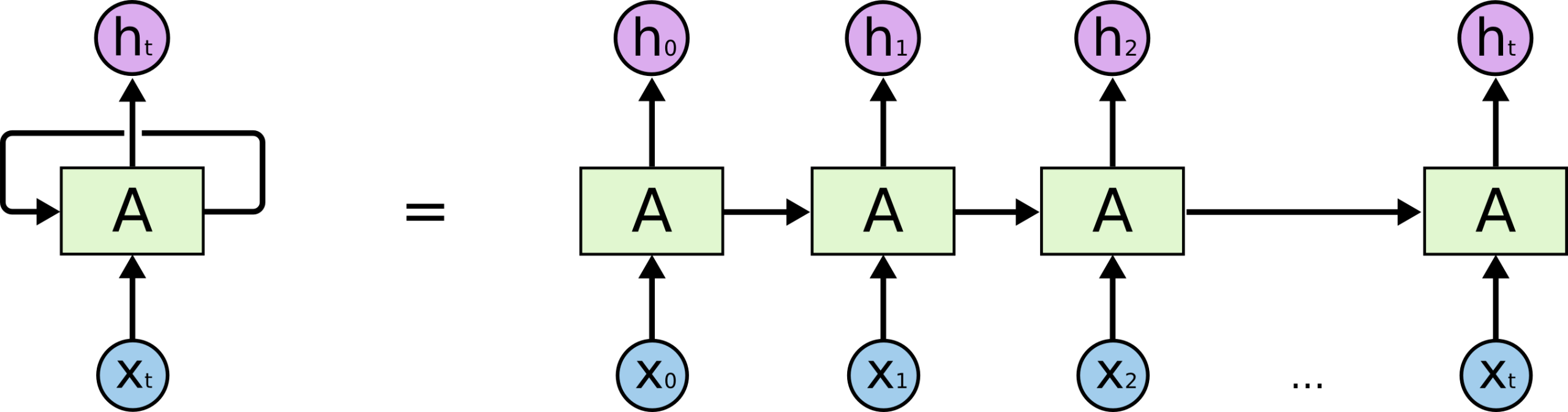
The core of RNN lies inrecurrent connections(Recurrent Connection), meaning the network's output depends not only on the current input but also on the inputs from all previous time steps. This structure enables RNNs to process sequential data of arbitrary length.
Traditional neural networks: Inputs and outputs are independent (e.g., image classification, where individual images are unrelated).
RNN: Throughrecurrent connections(Recurrent Connection), the hidden state from the previous step is passed to the next step, forming a "memory".
Input at each step = current data + hidden state from the previous step.
The output depends not only on the current input but also on the context from all previous steps.
Just as when reading a sentence, understanding the current word depends on previously read content (e.g., "He opened the __", you would predict "door" or "book").
Example
import numpy as np
class SimpleRNN:
def __init__(self, input_size, hidden_size):
self.Wx = np.random.randn(hidden_size, input_size) # Input weights
self.Wh = np.random.randn(hidden_size, hidden_size) # Hidden state weights
self.b = np.zeros((hidden_size, 1)) # Bias term
def forward(self, x, h_prev):
h_next = np.tanh(np.dot(self.Wx, x) + np.dot(self.Wh, h_prev) + self.b)
return h_next
How RNN Works
At each time step t, the RNN performs the following computations:
- Receives the current input xₜ and the hidden state hₜ₋₁ from the previous time step
- Computes the new hidden state hₜ = f(Wₕₕ·hₜ₋₁ + Wₓₕ·xₜ + b)
- Produces the output yₜ = g(Wₕᵧ·hₜ + c)
Where f and g are typically activation functions (such as tanh or softmax).
Advantages and Disadvantages of RNN
Advantages:
- Can handle variable-length sequences
- Theoretically can remember historical information of arbitrary length
- Parameter sharing (the same set of weights is used for all time steps)
Disadvantages:
- Vanishing/exploding gradient problem (difficult to learn long-term dependencies)
- Low computational efficiency (cannot process time steps in parallel)
Long Short-Term Memory (LSTM)
LSTM (Long Short-Term Memory) is an improved architecture of RNN, specifically designed to solve the long-term dependency problem of standard RNNs.
2.1 Core Structure of LSTM
LSTM introduces three gating mechanisms and a memory cell:
| Component | Function |
|---|---|
| Input gate | Controls the flow of new information |
| Forget gate | Decides which old information to discard |
| Output gate | Controls the amount of information to output |
| Memory cell | Stores long-term state |
Example
class LSTMCell:
def __init__(self, input_size, hidden_size):
# Combine the weights of all gates
self.W = np.random.randn(4*hidden_size, input_size+hidden_size)
self.b = np.random.randn(4*hidden_size, 1)
def forward(self, x, h_prev, c_prev):
combined = np.vstack((h_prev, x))
gates = np.dot(self.W, combined) + self.b
# Split to obtain each gate
f_gate = sigmoid(gates[:hidden_size]) # Forget gate
i_gate = sigmoid(gates[hidden_size:2*hidden_size]) # Input gate
o_gate = sigmoid(gates[2*hidden_size:3*hidden_size]) # Output gate
c_candidate = np.tanh(gates[3*hidden_size:]) # Candidate memory
# Update memory and hidden state
c_next = f_gate * c_prev + i_gate * c_candidate
h_next = o_gate * np.tanh(c_next)
return h_next, c_next
How LSTM Solves the Long-Term Dependency Problem
- Selective memory: The forget gate can decide to retain or discard specific information
- Gradient pathway: The memory cell provides a relatively direct path for gradient propagation
- Information protection: The stored memory content is not directly modified by the operations at every time step
Gated Recurrent Unit (GRU)
GRU (Gated Recurrent Unit) is a simplified version of LSTM that reduces the number of parameters while maintaining similar performance.
Core Structure of GRU
GRU merges certain components of LSTM:
| Component | Function |
|---|---|
| Update gate | Decides how much old information to retain |
| Reset gate | Decides how to combine new and old information |
| Candidate activation | New state computed based on the reset gate |
Example
class GRUCell:
def __init__(self, input_size, hidden_size):
self.W = np.random.randn(3*hidden_size, input_size+hidden_size)
self.b = np.random.randn(3*hidden_size, 1)
def forward(self, x, h_prev):
combined = np.vstack((h_prev, x))
gates = np.dot(self.W, combined) + self.b
# Split gating signals
z = sigmoid(gates[:hidden_size]) # Update gate
r = sigmoid(gates[hidden_size:2*hidden_size]) # Reset gate
h_candidate = np.tanh(np.dot(self.W[2*hidden_size:],
np.vstack((r*h_prev, x))) + self.b[2*hidden_size:]
# Update hidden state
h_next = (1-z)*h_prev + z*h_candidate
return h_next
GRU vs LSTM
| Feature | GRU | LSTM |
|---|---|---|
| Number of parameters | Fewer | More |
| Training speed | Faster | Slower |
| Memory cell | None | Yes |
| Number of gates | 2 | 3 |
| Performance | Better for small datasets | May be better for large datasets |
Bidirectional RNN (Bi-RNN)
Bidirectional RNN enhances sequence modeling capability by considering both past and future context information simultaneously.
Bidirectional RNN Architecture
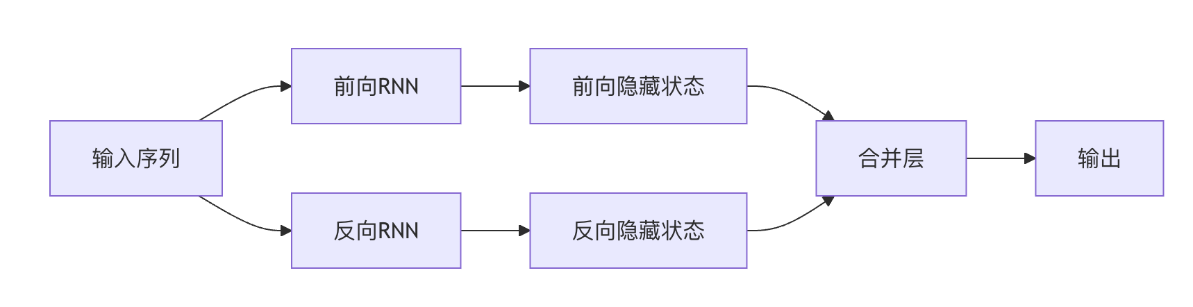
Bi-RNN consists of two independent RNN layers:
- Forward layer: processes the sequence in chronological order
- Backward layer: processes the sequence in reverse chronological order
The final output is a combination of the outputs from both directions (usually concatenation or summation).
Application Scenarios of Bidirectional RNN
- Natural language processing: Part-of-speech tagging, named entity recognition
- Speech recognition: Uses surrounding context to improve accuracy
- Bioinformatics: Protein structure prediction
- Time series forecasting: Considers historical and future trends
Bidirectional LSTM/GRU
In modern applications, bidirectional RNNs typically use LSTM or GRU as the basic unit:
Example
model.add(Bidirectional(LSTM(64))) # Create a bidirectional LSTM layer
Practical Exercises
Exercise 1: Implement a Simple RNN
Use Python and NumPy to implement a simple RNN capable of character-level text generation.
Exercise 2: LSTM Sentiment Analysis
Use Keras to build an LSTM-based movie review sentiment classifier.
Exercise 3: Bidirectional GRU Named Entity Recognition
Implement a bidirectional GRU model to identify entities such as person names and locations in text.
Exercise 4: Comparative Experiment
Compare the performance differences of Vanilla RNN, LSTM, and GRU on the same dataset.
Summary and Further Learning
RNN and its variants are powerful tools for processing sequential data. To master them deeply:
- Understand how gradients propagate in RNNs
- Learn how the attention mechanism enhances RNNs
- Explore the relationship between the Transformer architecture and RNNs
- Practice various sequence modeling tasks (machine translation, speech synthesis, etc.)