Keywords: Pipeline, Multiplier
A prominent advantage of hardware description languages is the parallelism of instruction execution. Multiple statements can process multiple signal data in parallel within the same clock cycle.
However, when data is input serially, the parallelism of instruction execution does not show its advantage. Moreover, in many cases some computations cannot be completed within one or two clock cycles. If each serial input data must wait until the previous computation is completed before starting the next computation, the efficiency is quite low. Pipelining is the solution to the low efficiency of serial data computation under multiple cycles.
Pipeline
The basic idea of pipelining is to decompose a repeated process into several sub-processes, each implemented by a dedicated functional unit. Multiple processing processes are staggered in time and pass through the functional stages sequentially, so that each sub-process can be executed in parallel with other sub-processes.
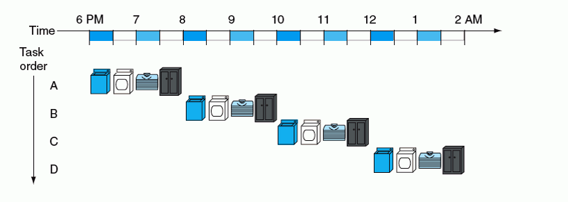
Suppose the process of washing clothes in a laundromat is divided into 4 stages: collecting clothes, washing, drying, and packing into cabinets. Each stage takes half an hour, so washing clothes once takes 2 hours.
Consider the worst case: the laundromat has only one washing machine, one dryer, and one cabinet. If a batch of clothes is delivered every half hour, and each time you have to wait 2 hours for the previous batch to finish washing, then washing 4 batches of clothes takes 8 hours.
The diagram is as follows:
Upgrade the equipment of this laundromat by introducing 4 sets of laundry equipment in total, and increase the staff to 4 people, each responsible for one stage of the laundry process. Therefore, each batch of clothes can be promptly put into different washing machines by the same person. Since the timing is staggered, each batch of clothes can be washed, dried, and packed into cabinets by the same people using different equipment and time periods (half an hour). The diagram is as follows.
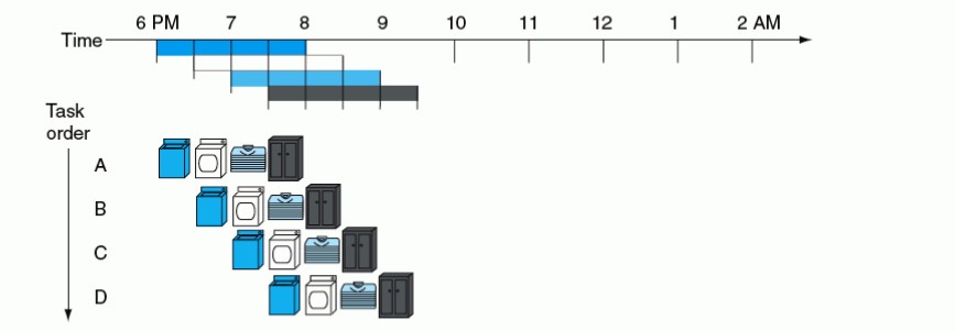
It can be seen that washing 4 batches of clothes only takes 3.5 hours, significantly improving efficiency.
In fact, after 2 hours, the first set of laundry equipment has completed the washing process and is idle. If a 5th batch of clothes is sent in at this time, the first set of equipment can start working again. By analogy, as long as clothes batches are continuously input, the 4 sets of laundry equipment can continuously complete the cleaning process for all clothes. Except for the first batch which takes 2 hours, a batch of clothes will be washed and completed every half hour thereafter.
The more batches of clothes there are, the more obvious the time saved. If there are N batches of clothes, the time required is (4+N) half-hours.
Of course, the upgraded laundry process also has disadvantages. The increase in equipment and staff raises the investment cost, reduces the remaining space in the laundromat, and makes the working state appear busier.
Similar to the washing process, the data processing path can also be viewed as a production line. Each digital processing unit on the path can be viewed as a stage, which introduces delay.
Pipeline design systematically divides the path into digital processing units (stages), and inserts registers between the processing units to temporarily store intermediate data. The divided units can execute in parallel by stage without affecting each other. Therefore, pipeline design can ultimately improve data throughput, that is, increase the data processing speed.
The disadvantage of pipeline design is that each processing stage requires additional registers to save intermediate calculation states, and multiple instructions executing in parallel will inevitably increase power consumption.
Next, a multiplier is designed, and a comparison is made between adopting and not adopting pipeline design.
General Multiplier Design
Introduction
Perhaps someone will ask, directly using the multiplication sign*to complete the multiplication of two numbers, isn't it faster and simpler?
If you have this doubt, it means your understanding of hardware description languages is still insufficient. As mentioned before, Verilog describes hardware circuits. When directly using the multiplication sign to complete the multiplication process, the compiler maps this multiplication expression to a default multiplier during compilation, but its structure is unknown.
For example, in FPGA design, an IP core can be directly called to generate a high-performance multiplier. When the bit width is small, the result can be output within one cycle; when the bit width is large, it can also be output in a pipelined manner. Under the premise that the requirements can be met, you can cautiously use*or directly call the IP to complete the multiplication operation.
But multiplier IP also has many defects, such as bit width limitations, unknown timing, etc. Especially using the multiplication sign can bury great hidden danger for the uncertainty of digital design.
In many cases, multiplication by constants is implemented in the form of shift-and-add, for example:
Example
A = (A<<1) + A ; // corresponds to A * 3
A = (A<<3) + (A<<2) + (A<<1) + A ; // corresponds to A * 15
A shift register and an adder can complete the operation of multiplying by 3. But multiplying by 15 requires 3 shift registers and 3 adders (of course, multiplying by 15 can also be done by shifting and subtracting).
Sometimes a digital circuit cannot complete the addition of multiple variables simultaneously within one cycle. Therefore, in digital design, the safest addition operation is to add only 2 data items at the same time; the worst design is to add 4 or more data items at the same time.
If the design contains an operation that adds 4 data items at the same time, then this part of the design is dangerous and may cause timing violations.
At this point, a pipelined multiplier with configurable design parameters and controllable timing becomes necessary.
Design Principle
Similar to decimal multiplication, the process of multiplying 13 and 5 is shown below:
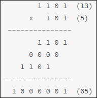
From this, it can be seen that the multiplicand is shifted and accumulated according to the corresponding bit of the multiplier, thereby completing the multiplication process.
Assuming only one accumulation can be completed per cycle, the minimum number of clocks for one multiplication is exactly the bit width of the multiplier. Therefore, it is recommended to use the number with the smaller bit width as the multiplier, so the calculation period is shorter.
Multiplier Design
Considering that each multiplication operation can only output one result (non-pipelined design), the design code is as follows.
Example
#(parameter N=4,
parameter M=4)
(
input clk,
input rstn,
input data_rdy , // data input enable
input [N-1:0] mult1, // multiplicand
input [M-1:0] mult2, // multiplier
output res_rdy , // data output enable
output [N+M-1:0] res // multiplication result
);
//calculate counter
reg [31:0] cnt ;
// multiplication cycle counter
wire [31:0] cnt_temp = (cnt == M)? 'b0 : cnt + 1'b1 ;
always @(posedge clk or negedge rstn) begin
if (!rstn) begin
cnt <= 'b0 ;
end
else if (data_rdy) begin // start counting when data is enabled
cnt <= cnt_temp ;
end
else if (cnt != 0 ) begin // prevent the input enable duration from being too short
cnt <= cnt_temp ;
end
else begin
cnt <= 'b0 ;
end
end
//multiply
reg [M-1:0] mult2_shift ;
reg [M+N-1:0] mult1_shift ;
reg [M+N-1:0] mult1_acc ;
always @(posedge clk or negedge rstn) begin
if (!rstn) begin
mult2_shift <= 'b0 ;
mult1_shift <= 'b0 ;
mult1_acc <= 'b0 ;
end
else if (data_rdy && cnt=='b0) begin // initialization
mult1_shift <= {{(N){1'b0}}, mult1} << 1 ;
mult2_shift <= mult2 >> 1 ;
mult1_acc <= mult2[0] ? {{(N){1'b0}}, mult1} : 'b0 ;
end
else if (cnt != M) begin
mult1_shift <= mult1_shift << 1 ; // multiplicand multiplied by 2
mult2_shift <= mult2_shift >> 1 ; // shift the multiplier right for easy judgment
// check whether the corresponding bit of the multiplier is 1; if 1, accumulate
mult1_acc <= mult2_shift[0] ? mult1_acc + mult1_shift : mult1_acc ;
end
else begin
mult2_shift <= 'b0 ;
mult1_shift <= 'b0 ;
mult1_acc <= 'b0 ;
end
end
//results
reg [M+N-1:0] res_r ;
reg res_rdy_r ;
always @(posedge clk or negedge rstn) begin
if (!rstn) begin
res_r <= 'b0 ;
res_rdy_r <= 'b0 ;
end
else if (cnt == M) begin
res_r <= mult1_acc ; // output the result at the end of the multiplication cycles
res_rdy_r <= 1'b1 ;
end
else begin
res_r <= 'b0 ;
res_rdy_r <= 'b0 ;
end
end
assign res_rdy = res_rdy_r;
assign res = res_r;
endmodule
testbench
Example
module test ;
parameter N = 8 ;
parameter M = 4 ;
reg clk, rstn;
//clock
always begin
clk = 0 ; #5 ;
clk = 1 ; #5 ;
end
//reset
initial begin
rstn = 1'b0 ;
#8 ; rstn = 1'b1 ;
end
//no pipeline
reg data_rdy_low ;
reg [N-1:0] mult1_low ;
reg [M-1:0] mult2_low ;
wire [M+N-1:0] res_low ;
wire res_rdy_low ;
// use a task for periodic stimulus
task mult_data_in ;
input [M+N-1:0] mult1_task, mult2_task ;
begin
wait(!test.u_mult_low.res_rdy) ; //not output state
@(negedge clk ) ;
data_rdy_low = 1'b1 ;
mult1_low = mult1_task ;
mult2_low = mult2_task ;
@(negedge clk ) ;
data_rdy_low = 1'b0 ;
wait(test.u_mult_low.res_rdy) ; //test the output state
end
endtask
//driver
initial begin
#55 ;
mult_data_in(25, 5 ) ;
mult_data_in(16, 10 ) ;
mult_data_in(10, 4 ) ;
mult_data_in(15, 7) ;
mult_data_in(215, 9) ;
end
mult_low #(.N(N), .M(M))
u_mult_low
(
.clk (clk),
.rstn (rstn),
.data_rdy (data_rdy_low),
.mult1 (mult1_low),
.mult2 (mult2_low),
.res_rdy (res_rdy_low),
.res (res_low));
//simulation finish
initial begin
forever begin
#100;
if ($time >= 10000) $finish ;
end
end
endmodule // test
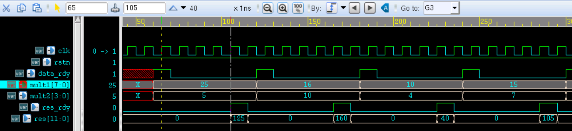
The simulation results are as follows.
As can be seen from the figure, the two input data items obtain the correct multiplication result after a delay of 4 cycles. Including the delay time of the intermediate data input, computing 4 multiplications takes about 20 clock cycles.
Pipelined Multiplier Design
Next, the intermediate states of the multiplication execution process are saved to enable pipelined operation. The design code is as follows.
The code file for a single accumulation calculation process is as follows (mult_cell.v):
Example
#(parameter N=4,
parameter M=4)
(
input clk,
input rstn,
input en,
input [M+N-1:0] mult1, // multiplicand
input [M-1:0] mult2, // multiplier
input [M+N-1:0] mult1_acci, // previous accumulation result
output reg [M+N-1:0] mult1_o, // saved value after multiplicand shift
output reg [M-1:0] mult2_shift, // saved value after multiplier shift
output reg [N+M-1:0] mult1_acco, // current accumulation result
output reg rdy );
always @(posedge clk or negedge rstn) begin
if (!rstn) begin
rdy <= 'b0 ;
mult1_o <= 'b0 ;
mult1_acco <= 'b0 ;
mult2_shift <= 'b0 ;
end
else if (en) begin
rdy <= 1'b1 ;
mult2_shift <= mult2 >> 1 ;
mult1_o <= mult1 << 1 ;
if (mult2[0]) begin
// accumulate if the corresponding bit of the multiplier is 1
mult1_acco <= mult1_acci + mult1 ;
end
else begin
mult1_acco <= mult1_acci ; // keep if the corresponding bit of the multiplier is 1
end
end
else begin
rdy <= 'b0 ;
mult1_o <= 'b0 ;
mult1_acco <= 'b0 ;
mult2_shift <= 'b0 ;
end
end
endmodule
Top-level Instantiation
Multiple module instantiations complete multiple accumulations. The code file is as follows (mult_man.v):
Example
#(parameter N=4,
parameter M=4)
(
input clk,
input rstn,
input data_rdy ,
input [N-1:0] mult1,
input [M-1:0] mult2,
output res_rdy ,
output [N+M-1:0] res );
wire [N+M-1:0] mult1_t [M-1:0] ;
wire [M-1:0] mult2_t [M-1:0] ;
wire [N+M-1:0] mult1_acc_t [M-1:0] ;
wire [M-1:0] rdy_t ;
// The first instantiation is equivalent to initialization; the generate statement cannot be used
mult_cell #(.N(N), .M(M))
u_mult_step0
(
.clk (clk),
.rstn (rstn),
.en (data_rdy),
.mult1 ({{(M){1'b0}}, mult1}),
.mult2 (mult2),
.mult1_acci ({(N+M){1'b0}}),
//output
.mult1_acco (mult1_acc_t[0]),
.mult2_shift (mult2_t[0]),
.mult1_o (mult1_t[0]),
.rdy (rdy_t[0]) );
// Multiple module instantiations use the generate statement
genvar i ;
generate
for(i=1; i<=M-1; i=i+1) begin: mult_stepx
mult_cell #(.N(N), .M(M))
u_mult_step
(
.clk (clk),
.rstn (rstn),
.en (rdy_t[i-1]),
.mult1 (mult1_t[i-1]),
.mult2 (mult2_t[i-1]),
// The previous accumulation result is used as the input for the next accumulation
.mult1_acci (mult1_acc_t[i-1]),
//output
.mult1_acco (mult1_acc_t[i]),
.mult1_o (mult1_t[i]), // multiplicand shift state transfer
.mult2_shift (mult2_t[i]), // multiplier shift state transfer
.rdy (rdy_t[i]) );
end
endgenerate
assign res_rdy = rdy_t[M-1];
assign res = mult1_acc_t[M-1];
endmodule
testbench
Add the following simulation description to the testbench of the non-pipelined multiplier design example to obtain the simulation results of the pipelined multiplication operation.
The 2 data channels are continuously and serially input, and a self-checking module is included to automatically determine the correctness of the multiplication results.
Example
reg [N-1:0] mult1 ;
reg [M-1:0] mult2 ;
wire res_rdy ;
wire [N+M-1:0] res ;
//driver
initial begin
#55 ;
@(negedge clk ) ;
data_rdy = 1'b1 ;
mult1 = 25; mult2 = 5;
#10 ; mult1 = 16; mult2 = 10;
#10 ; mult1 = 10; mult2 = 4;
#10 ; mult1 = 15; mult2 = 7;
mult2 = 7; repeat(32) #10 mult1 = mult1 + 1 ;
mult2 = 1; repeat(32) #10 mult1 = mult1 + 1 ;
mult2 = 15; repeat(32) #10 mult1 = mult1 + 1 ;
mult2 = 3; repeat(32) #10 mult1 = mult1 + 1 ;
mult2 = 11; repeat(32) #10 mult1 = mult1 + 1 ;
mult2 = 4; repeat(32) #10 mult1 = mult1 + 1 ;
mult2 = 9; repeat(32) #10 mult1 = mult1 + 1 ;
end
// shift the input data for convenient subsequent verification
reg [N-1:0] mult1_ref [M-1:0];
reg [M-1:0] mult2_ref [M-1:0];
always @(posedge clk) begin
mult1_ref[0] <= mult1 ;
mult2_ref[0] <= mult2 ;
end
genvar i ;
generate
for(i=1; i<=M-1; i=i+1) begin
always @(posedge clk) begin
mult1_ref[i] <= mult1_ref[i-1];
mult2_ref[i] <= mult2_ref[i-1];
end
end
endgenerate
// self-check
reg error_flag ;
always @(posedge clk) begin
# 1 ;
if (mult1_ref[M-1] * mult2_ref[M-1] != res && res_rdy) begin
error_flag <= 1'b1 ;
end
else begin
error_flag <= 1'b0 ;
end
end
//module instantiation
mult_man #(.N(N), .M(M))
u_mult
(
.clk (clk),
.rstn (rstn),
.data_rdy (data_rdy),
.mult1 (mult1),
.mult2 (mult2),
.res_rdy (res_rdy),
.res (res));
Simulation Results
The simulation results of the first few dozen clock cycles are as follows.
As can be seen from the figure, the simulation result check signal error_flag stays 0, indicating that the multiplier design is correct.
Data is continuously input serially under the clock drive. After a delay of 4 clock cycles, the multiplication output results are also continuously output on every clock cycle without extra delay, completing pipelined operation.
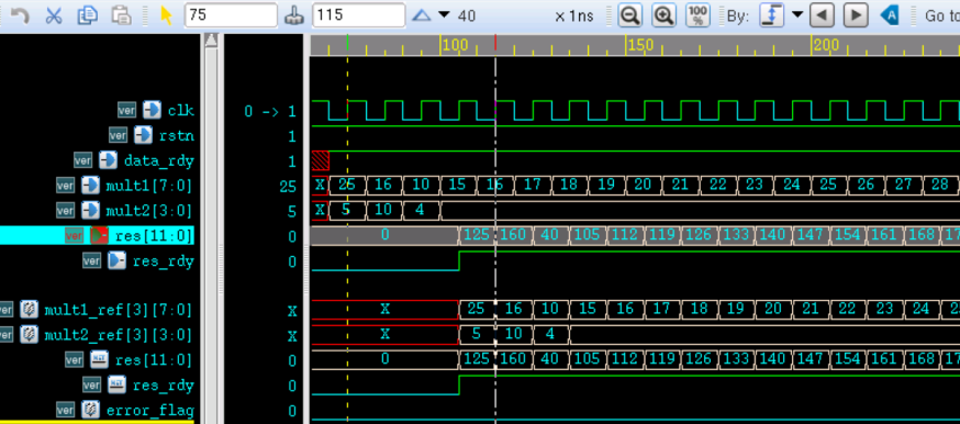
Compared with general multipliers that do not use pipelining, the multiplication efficiency has been greatly improved.
However, the register resources used by the pipelined multiplier are also about 4 times those of the previous non-pipelined one.
Therefore, whether a digital design adopts a pipelined design needs to be weighed in terms of both resources and efficiency.
Source Code Download
Download