Sklearn Application Examples
The Iris Dataset is one of the most classic introductory datasets in machine learning.
The Iris dataset contains three iris species (Setosa, Versicolor, Virginica) and 4 features for each flower: sepal length, sepal width, petal length, and petal width.
Next, our task is to predict the iris species based on these features.
The case in this chapter will cover steps such as data loading, visualization, feature selection, data preprocessing, building a classification model, model evaluation, and optimization.
1. Data Loading and Visualization
Data Loading
First, load the Iris dataset. scikit-learn provides an interface to directly load the Iris dataset.
Example
import pandas as pd
# Load the Iris dataset
data = load_iris()
# Convert to DataFrame for easy viewing
df = pd.DataFrame(data.data, columns=data.feature_names)
df['target'] = data.target
df['species'] = df['target'].apply(lambda x: data.target_names[x])
# View the first few rows of data
print(df.head())
Output:
   sepal length (cm)  sepal width (cm)  petal length (cm)  petal width (cm)  target species
0                 5.1               3.5                1.4               0.2       0   setosa
1                 4.9               3.0                1.4               0.2       0   setosa
2                 4.7               3.2                1.3               0.2       0   setosa
3                 4.6               3.1                1.5               0.2       0   setosa
4                 5.0               3.6                1.4               0.2       0   setosa
At this point, the data has been loaded successfully, and we can see the features and corresponding flower species for each record.
Data Visualization
To better understand the data, we can visualize the relationships between different features. We can use the matplotlib and seaborn libraries for visualization.
Example
import pandas as pd
import seaborn as sns
import matplotlib.pyplot as plt
# Load the Iris dataset
data = load_iris()
# Convert to DataFrame for easy viewing
df = pd.DataFrame(data.data, columns=data.feature_names)
df['target'] = data.target
df['species'] = df['target'].apply(lambda x: data.target_names[x])
# Plot the relationships between features
sns.pairplot(df, hue="species")
plt.show()
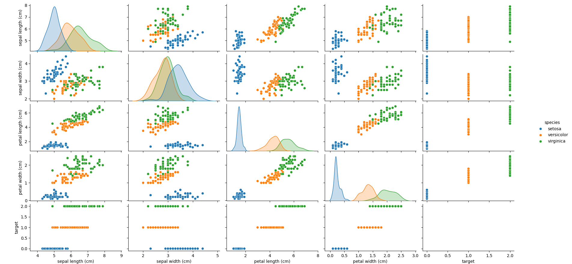
pairplot will draw a scatter plot matrix between features, using different colors to identify different iris species. This helps us understand the distribution of each feature and the relationships between them.
The displayed figure is as follows:
Heatmap to Visualize Correlations Between Features
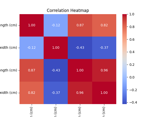
Through the heatmap, we can view the correlations between features. Stronger correlations can help us make better choices when modeling.
Example
import pandas as pd
import seaborn as sns
import matplotlib.pyplot as plt
# Load the Iris dataset
data = load_iris()
# Convert to DataFrame for easy viewing
df = pd.DataFrame(data.data, columns=data.feature_names)
df['target'] = data.target
df['species'] = df['target'].apply(lambda x: data.target_names[x])
# Plot the relationships between features
correlation_matrix = df.drop(columns=['target', 'species']).corr()
sns.heatmap(correlation_matrix, annot=True, cmap="coolwarm", fmt=".2f")
plt.title("Correlation Heatmap")
plt.show()
The displayed figure is as follows:
2. Feature Selection and Data Preprocessing
Data Preprocessing
In machine learning, data preprocessing is a very important step.
For the Iris dataset, the feature values are already numeric, so not much preprocessing is needed. However, we can standardize the data to improve the model training effect.
Example
# Extract features and labels
X = df.drop(columns=['target', 'species'])
y = df['target']
# Standardize features
scaler = StandardScaler()
X_scaled = scaler.fit_transform(X)
The purpose of standardization is to make each feature have a mean of 0 and a variance of 1, which is very important for some distance-based models such as KNN and SVM.
Feature Selection
Although the features of the Iris dataset are relatively simple, in real-world problems we sometimes need to reduce feature dimensions through feature selection to improve model performance.
We can use methods such as SelectKBest or Recursive Feature Elimination (RFE).
For example, use SelectKBest to select the 2 features most relevant to the labels:
Example
# Use chi-square test to select the 2 most relevant features
selector = SelectKBest(f_classif, k=2)
X_new = selector.fit_transform(X_scaled, y)
# Print the selected features
selected_features = selector.get_support(indices=True)
print("Selected features:", X.columns[selected_features])
This will select the 2 features with the highest correlation to the target labels.
3. Build a Classification Model: Use Decision Tree or SVM for Classification
Using the Decision Tree Classifier
We will first try using a Decision Tree model for classification.
Example
from sklearn.tree import DecisionTreeClassifier
from sklearn.metrics import accuracy_score
# Split the dataset
X_train, X_test, y_train, y_test = train_test_split(X_scaled, y, test_size=0.2, random_state=42)
# Initialize the decision tree classifier
model_dt = DecisionTreeClassifier(random_state=42)
# Train the model
model_dt.fit(X_train, y_train)
# Predict
y_pred_dt = model_dt.predict(X_test)
# Evaluate the model
accuracy_dt = accuracy_score(y_test, y_pred_dt)
print(f"Decision Tree Accuracy: {accuracy_dt:.4f}")
Classifying Using Support Vector Machine (SVM)
Next, we can try using Support Vector Machine (SVM) for classification.
Example
# Initialize SVM classifier
model_svm = SVC(kernel='linear', random_state=42)
# Train the model
model_svm.fit(X_train, y_train)
# Predict
y_pred_svm = model_svm.predict(X_test)
# Evaluate the model
accuracy_svm = accuracy_score(y_test, y_pred_svm)
print(f"SVM Accuracy: {accuracy_svm:.4f}")
4. Evaluate and Optimize the Model
Model Evaluation
In addition to accuracy, we can also use other evaluation metrics such as confusion matrix, precision, recall, and F1 score.
Example
# Confusion matrix
cm = confusion_matrix(y_test, y_pred_dt)
print("Confusion Matrix (Decision Tree):")
print(cm)
# Precision, recall, F1 score
report = classification_report(y_test, y_pred_dt)
print("Classification Report (Decision Tree):")
print(report)
Grid Search Tuning
To optimize the model, we can use grid search (GridSearchCV) to tune the model hyperparameters and find the best parameter combination.
Example
# Define the parameter grid for the decision tree
param_grid = {
'max_depth': [3, 5, 10, None],
'min_samples_split': [2, 5, 10],
'min_samples_leaf': [1, 2, 4]
}
# Initialize GridSearchCV
grid_search = GridSearchCV(estimator=DecisionTreeClassifier(random_state=42), param_grid=param_grid, cv=5)
# Train the grid search
grid_search.fit(X_train, y_train)
# Get the best parameters and best model
print("Best Parameters:", grid_search.best_params_)
best_model = grid_search.best_estimator_
# Predict and evaluate
y_pred_optimized = best_model.predict(X_test)
accuracy_optimized = accuracy_score(y_test, y_pred_optimized)
print(f"Optimized Decision Tree Accuracy: {accuracy_optimized:.4f}")
Through grid search, we can find the decision tree parameters that best fit the current data and improve the model's prediction accuracy.
Cross-Validation
To further evaluate the stability of the model, we can use cross-validation to assess its performance.
Example
# Perform 5-fold cross-validation
cross_val_scores = cross_val_score(best_model, X_scaled, y, cv=5)
print(f"Cross-validation Scores: {cross_val_scores}")
print(f"Mean CV Accuracy: {cross_val_scores.mean():.4f}")
Cross-validation helps us evaluate the model's performance on different data subsets and avoid overfitting.
5. Complete Code
The following is a complete code example covering steps such as loading the Iris dataset, data preprocessing, feature selection, building classification models, model evaluation, and optimization. We will use decision tree and SVM classifiers, and optimize the model hyperparameters through grid search.Example
import numpy as np
import pandas as pd
import seaborn as sns
import matplotlib.pyplot as plt
from sklearn.datasets import load_iris
from sklearn.model_selection import train_test_split, GridSearchCV, cross_val_score
from sklearn.preprocessing import StandardScaler
from sklearn.tree import DecisionTreeClassifier
from sklearn.svm import SVC
from sklearn.metrics import accuracy_score, classification_report, confusion_matrix
# 1. Data loading
# Load the Iris dataset
data = load_iris()
# Convert to DataFrame for easy viewing
df = pd.DataFrame(data.data, columns=data.feature_names)
df['target'] = data.target
df['species'] = df['target'].apply(lambda x: data.target_names[x])
# View the first few rows of data
print("Data preview:")
print(df.head())
# 2. Data visualization
# Plot the relationships between features
sns.pairplot(df, hue="species")
plt.show()
# Plot a heatmap to view correlations between features
correlation_matrix = df.drop(columns=['target', 'species']).corr()
sns.heatmap(correlation_matrix, annot=True, cmap="coolwarm", fmt=".2f")
plt.title("Correlation Heatmap")
plt.show()
# 3. Feature selection and data preprocessing
# Extract features and labels
X = df.drop(columns=['target', 'species'])
y = df['target']
# Standardize data
scaler = StandardScaler()
X_scaled = scaler.fit_transform(X)
# 4. Build classification models
# Split the dataset
X_train, X_test, y_train, y_test = train_test_split(X_scaled, y, test_size=0.2, random_state=42)
# Use decision tree classifier
model_dt = DecisionTreeClassifier(random_state=42)
model_dt.fit(X_train, y_train)
# Predict
y_pred_dt = model_dt.predict(X_test)
# Output the accuracy of the decision tree
accuracy_dt = accuracy_score(y_test, y_pred_dt)
print(f"Decision Tree Accuracy: {accuracy_dt:.4f}")
# Use Support Vector Machine (SVM) classifier
model_svm = SVC(kernel='linear', random_state=42)
model_svm.fit(X_train, y_train)
# Predict
y_pred_svm = model_svm.predict(X_test)
# Output the accuracy of SVM
accuracy_svm = accuracy_score(y_test, y_pred_svm)
print(f"SVM Accuracy: {accuracy_svm:.4f}")
# 5. Model evaluation
# Decision tree model evaluation
print("\nDecision Tree Classification Report:")
print(classification_report(y_test, y_pred_dt))
print("\nDecision Tree Confusion Matrix:")
print(confusion_matrix(y_test, y_pred_dt))
# SVM model evaluation
print("\nSVM Classification Report:")
print(classification_report(y_test, y_pred_svm))
print("\nSVM Confusion Matrix:")
print(confusion_matrix(y_test, y_pred_svm))
# 6. Grid search tuning
# Define the parameter grid for the decision tree
param_grid = {
'max_depth': [3, 5, 10, None],
'min_samples_split': [2, 5, 10],
'min_samples_leaf': [1, 2, 4]
}
# Initialize GridSearchCV
grid_search = GridSearchCV(estimator=DecisionTreeClassifier(random_state=42), param_grid=param_grid, cv=5)
grid_search.fit(X_train, y_train)
# Get the best parameters and best model
print("\nBest Parameters from GridSearchCV (Decision Tree):")
print(grid_search.best_params_)
# Use the best model for prediction
best_model = grid_search.best_estimator_
y_pred_optimized = best_model.predict(X_test)
# Output the optimized decision tree accuracy
accuracy_optimized = accuracy_score(y_test, y_pred_optimized)
print(f"Optimized Decision Tree Accuracy: {accuracy_optimized:.4f}")
# 7. Cross-validation
# Perform 5-fold cross-validation
cross_val_scores = cross_val_score(best_model, X_scaled, y, cv=5)
print("\nCross-validation Scores (Optimized Decision Tree):")
print(cross_val_scores)
print(f"Mean CV Accuracy: {cross_val_scores.mean():.4f}")
Code explanation:
Data loading:
- Use
load_iris()load the Iris dataset, and convert the data intoDataFrameformat for viewing and analysis.
- Use
Data visualization:
- Use
seabornofpairplotto plot the scatter plot matrix between features, and useheatmapto plot the correlation heatmap between features.
- Use
Feature selection and data preprocessing:
- Extract features (
X) and labels (y), and standardize the feature data so that each feature has a mean of 0 and a variance of 1.
- Extract features (
Build classification model:
- Use
DecisionTreeClassifierandSVCTrain decision tree classifier and support vector machine classifier respectively, and evaluate their accuracy on the test set.
- Use
Model evaluation:
- Use
classification_reportandconfusion_matrixOutput detailed evaluation metrics of the model, including precision, recall, F1 score, and confusion matrix.
- Use
Grid search tuning:
- Use
GridSearchCVPerform hyperparameter tuning on the decision tree model, find the best hyperparameter combination, and output the optimized model accuracy.
- Use
Cross-validation:
- Use
cross_val_scorePerform 5-fold cross-validation to evaluate the stability and performance of the optimized decision tree model.
- Use
The output is as follows:
数据预览:
   sepal length (cm)  sepal width (cm)  petal length (cm)  petal width (cm)  target species
0                 5.1               3.5                1.4               0.2       0   setosa
1                 4.9               3.0                1.4               0.2       0   setosa
2                 4.7               3.2                1.3               0.2       0   setosa
3                 4.6               3.1                1.5               0.2       0   setosa
4                 5.0               3.6                1.4               0.2       0   setosa

Decision Tree Accuracy: 1.0000
SVM Accuracy: 1.0000

Decision Tree Classification Report:
              precision    recall  f1-score   support

           0       1.00      1.00      1.00         9
           1       1.00      1.00      1.00         8
           2       1.00      1.00      1.00         8

    accuracy                           1.00        25
   macro avg       1.00      1.00      1.00        25
weighted avg       1.00      1.00      1.00        25

Decision Tree Confusion Matrix:
[[9 0 0]
 [0 8 0]
 [0 0 8]]

SVM Classification Report:
              precision    recall  f1-score   support

           0       1.00      1.00      1.00         9
           1       1.00      1.00      1.00         8
           2       1.00      1.00      1.00         8

    accuracy                           1.00        25
   macro avg       1.00      1.00      1.00        25
weighted avg       1.00      1.00      1.00        25

SVM Confusion Matrix:
[[9 0 0]
 [0 8 0]
 [0 0 8]]

Best Parameters from GridSearchCV (Decision Tree):
{'max_depth': 5, 'min_samples_leaf': 1, 'min_samples_split': 2}

Optimized Decision Tree Accuracy: 1.0000

Cross-validation Scores (Optimized Decision Tree):
[1.         1.         1.         1.         1.        ]
Mean CV Accuracy: 1.0000
Other extensions