SciPy Spatial Data

Spatial data, also known as geometric data, is used to represent information about various aspects of objects such as position, shape, size distribution, etc., for example, points on coordinates.

SciPy handles spatial data through the scipy.spatial module, such as determining whether a point is inside a boundary, calculating the closest point around a given point, and all points within a given distance.

Triangulation

Triangulation, in trigonometry and geometry, is a method of measuring the distance to a target by measuring the angles between the target point and the known endpoints of a fixed baseline.

Triangulation of a polygon is the division of the polygon into multiple triangles, and we can use these triangles to calculate the area of the polygon.

A known fact in topology tells us that any surface has a triangulation.

Suppose there is a triangulation on a surface. Let the total number of vertices of all triangles be denoted as p (common vertices are counted only once), the number of edges as a, and the number of triangles as n. Then e = p - a + n is a topological invariant of the surface. That is, no matter what triangulation is used, e always yields the same value. e is called the Euler characteristic.

The method for triangulating a set of points is Delaunay() triangulation.

The output result is shown in the figure below:

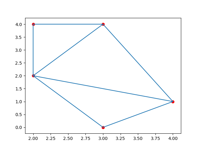
Note:The ids of the triangle vertices are stored in the simplices attribute of the triangulation object.

Convex Hull

Convex Hull is a concept in computational geometry (graphics).

In a real vector space V, for a given set X, the intersection S of all convex sets containing X is called the convex hull of X. The convex hull of X can be constructed using convex combinations of all points (X1, ...Xn) in X.

We can use the ConvexHull() method to create a convex hull.

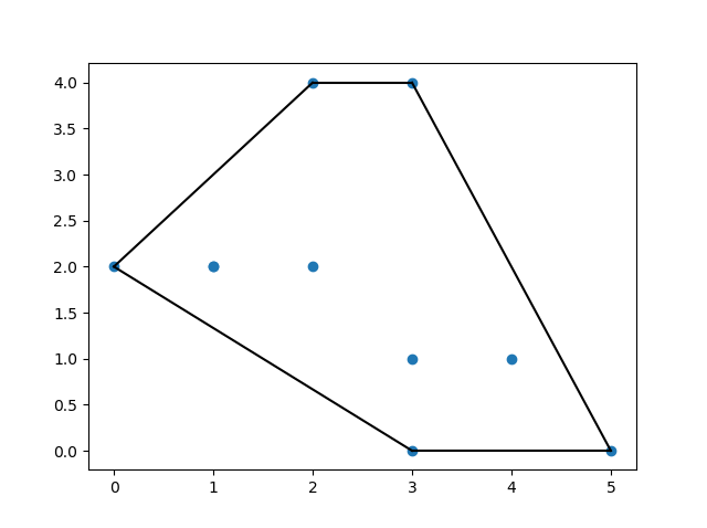
The output result is shown in the figure below:

K-D Tree

kd-tree (abbreviation of k-dimensional tree) is a tree data structure that stores instance points in k-dimensional space for fast retrieval. It is mainly used for searching key data in multidimensional space (e.g., range search and nearest neighbor search).

K-D trees can be used in various applications, such as multidimensional key search (range search and nearest neighbor search).

Nearest neighbor search is used to find the point in the tree closest to the input point.

KDTree()The method returns a KDTree object.

query()The method returns the nearest neighbor distance and the nearest neighbor position.

The output result is shown in the figure below:

(2.0, 0)

Distance Matrix

In mathematics, a distance matrix is a matrix (two-dimensional array) whose elements are the distances between points. Therefore, given N points in Euclidean space, its distance matrix is a matrix with non-negative real numbers as elements.N×NThe symmetric matrix. Distance matrix and adjacency matrix are similar in concept, the difference being that the latter only contains whether there is an edge between elements (points), and does not contain information about the distance of the connection between elements (points). Therefore, a distance matrix can be seen as a weighted form of an adjacency matrix.

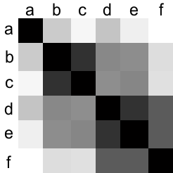
For example, we analyze the following two-dimensional points a to f. Here, we take the Euclidean metric between the pixels where the points are located as the distance metric.

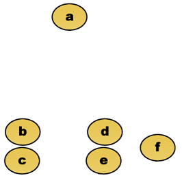
Its distance matrix is:

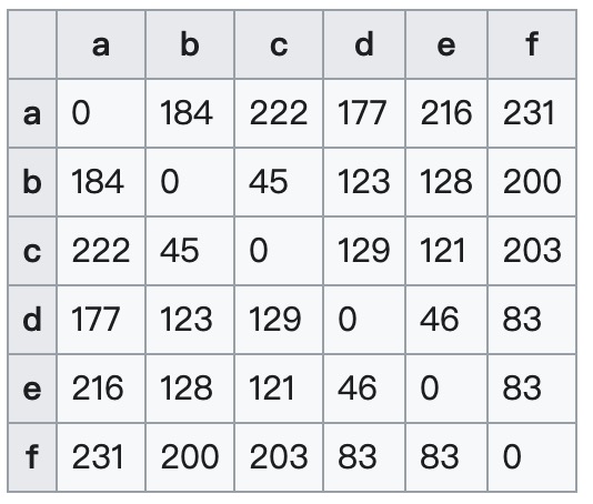
These data of the distance matrix can be further viewed as a heat map in graphical representation (as shown in the figure below), where black represents zero distance and white represents the maximum distance.

In bioinformatics, distance matrices are used to represent protein structures independent of coordinate systems, as well as the distances between two sequences in sequence space. These representations are used in structure alignment, sequence alignment, and in determining protein structures in NMR, X-ray, and crystallography.

Euclidean Distance

In mathematics, the Euclidean distance or Euclidean metric is the "ordinary" (i.e., straight-line) distance between two points in Euclidean space. With this distance, Euclidean space becomes a metric space. The associated norm is called the Euclidean norm. Earlier literature refers to it as the Pythagorean metric.

The Euclidean metric (also called Euclidean distance) is a commonly used definition of distance, referring to the actual distance between two points in m-dimensional space, or the natural length of a vector (i.e., the distance from the point to the origin). In two-dimensional and three-dimensional space, the Euclidean distance is the actual distance between two points.

The following example looks at the Euclidean distance between given points:

The output result is shown in the figure below:

9.21954445729

Manhattan Distance

Taxicab geometry or Manhattan Distance is a term coined by Hermann Minkowski in the nineteenth century. It is a geometric term used in metric spaces to indicate the sum of the absolute axial distances between two points in a standard coordinate system.

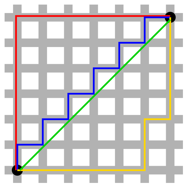
Manhattan distance only allows movement in the four directions up, down, left, and right, and the Manhattan distance between two points is the shortest distance between them.

Manhattan vs. Euclidean distance: The red, blue, and yellow lines respectively indicate that all Manhattan distances have the same length (12), while the green line indicates that the Euclidean distance has a length of 6×√2 ≈ 8.48.

The following example calculates the Manhattan distance between the given points:

The output result is:

11

Cosine Distance

Cosine distance, also known as cosine similarity, measures the similarity between two vectors by measuring the cosine of the angle between them.

The cosine of a 0-degree angle is 1, while the cosine of any other angle is not greater than 1, and its minimum value is -1.

The following example calculates the cosine distance between points A and B:

The output result is:

0.019419324309079777

Hamming Distance

In information theory, the Hamming distance between two equal-length strings is the number of positions at which the corresponding characters differ. In other words, it is the number of characters that need to be replaced to transform one string into the other.

The Hamming weight is the Hamming distance between a string and a zero string of the same length. In other words, it is the number of non-zero elements in the string: for a binary string, it is the number of 1s, so the Hamming weight of 11101 is 4.

• 1011101and1001001The Hamming distance between them is 2.
• 2143896and2233796The Hamming distance between them is 3.
• "toned"and"roses"The Hamming distance between them is 3.

The following example calculates the Hamming distance between two points:

The output result is:

0.666666666667