SciPy Graph Structure
Graph structure is one of the most powerful frameworks in algorithmics.
A graph is a collection of nodes and edges of various relationships. Nodes are vertices corresponding to objects, and edges are connections between objects.
SciPy provides the scipy.sparse.csgraph module to handle graph structures.
Adjacency Matrix
An adjacency matrix is a matrix that represents the adjacency relationships between vertices.
The logical structure of an adjacency matrix is divided into two parts: the V and E sets, where V is vertices, E is edges. Edges sometimes have weights, representing the connection strength between nodes.
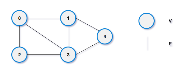
A one-dimensional array is used to store all vertex data in the graph, and a two-dimensional array is used to store the data of relationships between vertices (edges or arcs). This two-dimensional array is called an adjacency matrix.
Look at the following example:

The vertices are A, B, C, and the edge weights are 1 and 2.
A and B are connected with weight 1.
A and C are connected with weight 2.
C and B are not connected.
This adjacency matrix can be represented as the following two-dimensional array:
     A B C
   A:[0 1 2]
   B:[1 0 0]
   C:[2 0 0]
Adjacency matrices are further divided into directed graph adjacency matrices and undirected graph adjacency matrices.
An undirected graph is a bidirectional relationship, and edges have no direction:
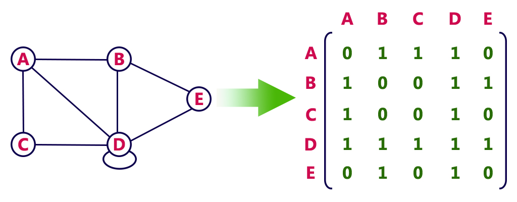
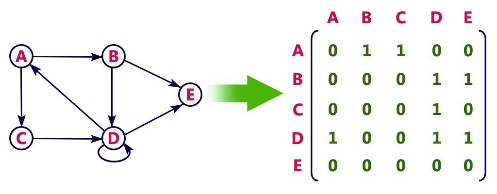
Note:The D node in the two figures above is a self-loop. A self-loop means that both ends of an edge are the same node.
Connected Components
Use the connected_components() method to view all connected components.
Example
from scipy.sparse.csgraph import connected_components
from scipy.sparse import csr_matrix
arr = np.array([
[0, 1, 2],
[1, 0, 0],
[2, 0, 0]
])
newarr = csr_matrix(arr)
print(connected_components(newarr))
The output of the above code is:
(1, array([0, 0, 0], dtype=int32))
Dijkstra -- Shortest Path Algorithm
Dijkstra's shortest path algorithm is used to compute the shortest paths from one node to all other nodes.
SciPy uses the dijkstra() method to compute the shortest path from one element to other elements.
The dijkstra() method can set the following parameters:- return_predecessors:A boolean value. Set to True to traverse all paths; if you do not want to traverse all paths, set it to False.
- indices:The index of the element, returning all paths from that element.
- limit:The maximum weight of the paths.
Example
Find the shortest path from element 1 to element 2:
from scipy.sparse.csgraph import dijkstra
from scipy.sparse import csr_matrix
arr = np.array([
[0, 1, 2],
[1, 0, 0],
[2, 0, 0]
])
newarr = csr_matrix(arr)
print(dijkstra(newarr, return_predecessors=True, indices=0))
The output of the above code is:
(array([ 0., 1., 2.]), array([-9999, 0, 0], dtype=int32))
Floyd Warshall -- Floyd's Algorithm
Floyd's algorithm is an algorithm for solving the shortest path between any two points.
SciPy uses the floyd_warshall() method to find the shortest path between all pairs of elements.
Example
Find the shortest paths between all pairs of elements:
from scipy.sparse.csgraph import floyd_warshall
from scipy.sparse import csr_matrix
arr = np.array([
[0, 1, 2],
[1, 0, 0],
[2, 0, 0]
])
newarr = csr_matrix(arr)
print(floyd_warshall(newarr, return_predecessors=True))
The output of the above code is:
(array([[ 0.,  1.,  2.],
       [ 1.,  0.,  3.],
       [ 2.,  3.,  0.]]), array([[-9999,     0,     0],
       [    1, -9999,     0],
       [    2,     0, -9999]], dtype=int32))
Bellman Ford -- Bellman-Ford Algorithm
The Bellman-Ford algorithm is an algorithm for solving the shortest path between any two points.
SciPy uses the bellman_ford() method to find the shortest path between all pairs of elements. It can generally be used in any graph, including directed graphs and graphs with negative weight edges.
Example
Use a graph with negative weight edges to find the shortest path from element 1 to element 2:
from scipy.sparse.csgraph import bellman_ford
from scipy.sparse import csr_matrix
arr = np.array([
[0, -1, 2],
[1, 0, 0],
[2, 0, 0]
])
newarr = csr_matrix(arr)
print(bellman_ford(newarr, return_predecessors=True, indices=0))
The output of the above code is:
(array([ 0., -1., 2.]), array([-9999, 0, 0], dtype=int32))
Depth First Order
The depth_first_order() method returns the depth-first traversal order from a node.
It can accept the following parameters:
- Graph
- The element from which the graph traversal starts
Example
Given an adjacency matrix, return the depth-first traversal order:
from scipy.sparse.csgraph import depth_first_order
from scipy.sparse import csr_matrix
arr = np.array([
[0, 1, 0, 1],
[1, 1, 1, 1],
[2, 1, 1, 0],
[0, 1, 0, 1]
])
newarr = csr_matrix(arr)
print(depth_first_order(newarr, 1))
The output of the above code is:
(array([1, 0, 3, 2], dtype=int32), array([ 1, -9999, 1, 0], dtype=int32))
Breadth First Order
The breadth_first_order() method returns the breadth-first traversal order from a node.
It can accept the following parameters:
- Graph
- The element from which the graph traversal starts
Example
Given an adjacency matrix, return the breadth-first traversal order:
from scipy.sparse.csgraph import breadth_first_order
from scipy.sparse import csr_matrix
arr = np.array([
[0, 1, 0, 1],
[1, 1, 1, 1],
[2, 1, 1, 0],
[0, 1, 0, 1]
])
newarr = csr_matrix(arr)
print(breadth_first_order(newarr, 1))
The output of the above code is:
(array([1, 0, 2, 3], dtype=int32), array([ 1, -9999, 1, 1], dtype=int32))Other Extensions