Python Quantitative Backtesting
Backtesting is the process of simulating and evaluating a trading strategy on historical market data.
In quantitative finance and algorithmic trading, backtesting is a key step used to evaluate the performance of a trading strategy on past market behavior.
Through backtesting, traders can understand how their strategies perform under different market conditions, and optimize and improve them.
Backtesting typically includes the following steps:
Define the trading strategy:Determine the rules for when to buy, sell, or hold positions. This may involve various strategies such as technical indicators, moving average strategies, trend following, arbitrage, and more.
Obtain historical data:Retrieve past market data, including prices, trading volumes, and other information for financial instruments such as stocks, futures, and foreign exchange.
Simulate trading:Based on the defined strategy, simulate executing trades on historical data. This includes determining when to buy or sell, and calculating the gains and losses of each trade.
Calculate performance metrics:Based on the backtest results, calculate various performance metrics such as annualized return, maximum drawdown, Sharpe ratio, etc., to evaluate the strategy's performance.
Optimize the strategy:If the backtest results are unsatisfactory, traders can optimize the strategy by adjusting parameters or modifying rules, and then re-run the backtest.
Look-ahead bias testing:A key issue in backtesting is preventing the leakage of future data. Look-ahead bias testing ensures that only a portion of historical data is used when designing and evaluating a strategy, to simulate the situation in actual trading where only known information can be used.
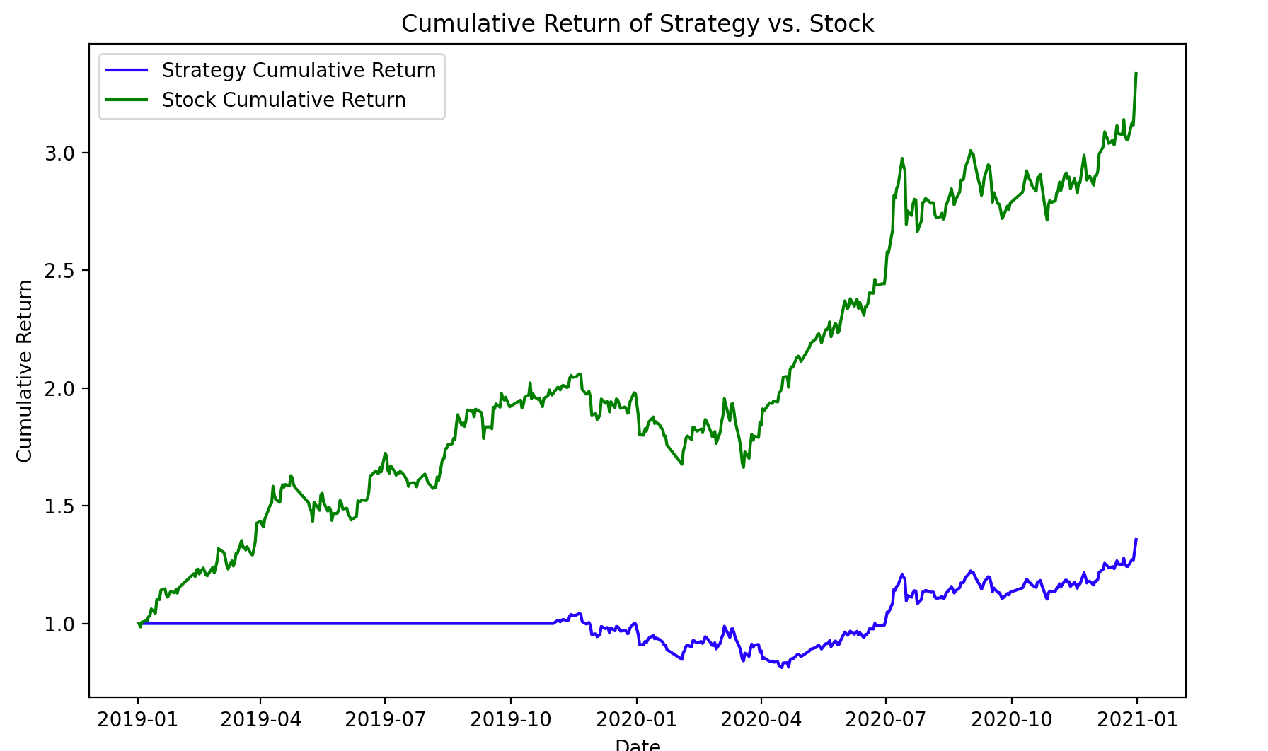
Next, here is example code for backtesting a simple moving average crossover strategy:
Example
import pandas as pd
import matplotlib.pyplot as plt
# Get stock data
symbol = "600519.SS" # Stock code for Moutai
start_date = "2019-01-01"
end_date = "2021-01-01"
data = yf.download(symbol, start=start_date, end=end_date)
# Calculate moving average
data['SMA_50'] = data['Close'].rolling(window=50).mean()
data['SMA_200'] = data['Close'].rolling(window=200).mean()
# Initialize crossover signal column
data['Signal'] = 0
# Calculate crossover signals
data.loc[data['SMA_50'] > data['SMA_200'], 'Signal'] = 1
data.loc[data['SMA_50'] < data['SMA_200'], 'Signal'] = -1
# Calculate daily returns
data['Daily_Return'] = data['Close'].pct_change()
# Calculate the return of the strategy signal (shift(1) is used to avoid look-ahead bias)
data['Strategy_Return'] = data['Signal'].shift(1) * data['Daily_Return']
# Calculate cumulative returns
data['Cumulative_Return'] = (1 + data['Strategy_Return']).cumprod()
# Plot cumulative return curve
plt.figure(figsize=(10, 6))
plt.plot(data['Cumulative_Return'], label='Strategy Cumulative Return', color='b')
plt.plot(data['Close'] / data['Close'].iloc[0], label='Stock Cumulative Return', color='g')
plt.title("Cumulative Return of Strategy vs. Stock")
plt.xlabel("Date")
plt.ylabel("Cumulative Return")
plt.legend()
plt.show()
Executing the above code produces the following output: