Three-way sorting algorithm
Three-way sorting algorithm(Three-Way Partitioning) is a special variant of quicksort, optimized specifically for arrays containing many duplicate elements. Its core idea is to divide the array into three parts in a single partitioning pass, rather than the traditional two parts.
Three-way quicksort is a further improved version of two-way quicksort. The three-way sorting algorithm divides the data to be sorted into three parts: less than v, equal to v, and greater than v, where v is the pivot. In this way, among the three parts, the data equal to v no longer needs to be sorted in the next recursion, and the data less than v or greater than v will not have a situation where one side is particularly large. With this approach, the three-way quicksort algorithm has better performance.
Imagine you have a large bucket of mixed colored marbles with three colors: red, white, and blue. Your task is to separate them quickly so that all the red marbles are on the left, the white ones in the middle, and the blue ones on the right. The three-way partitioning algorithm is the sorting master for solving this kind of problem.
Traditional quicksort vs. three-way quicksort
Let's use a simple table to compare the differences between the two:
| Features | Traditional quicksort | Three-way quicksort |
|---|---|---|
| Number of partitions | 2 (less than pivot, greater than pivot) | 3 (less than pivot, equal to pivot, greater than pivot) |
| Handling duplicate elements | Less efficient; duplicate elements may be compared and swapped multiple times | Extremely efficient, duplicate elements are handled together |
| Time complexity | Average O(n log n), worst O(n²) | Average O(n log n), worst O(n²) |
| Space complexity | O(log n) (recursion stack) | O(log n) (recursion stack) |
| Applicable scenarios | General-purpose sorting, low element duplication rate | High duplication of elements, such as color sorting and score segmentation |
Applicability
The time and space complexity are the same as randomized quicksort.
The three-way quicksort algorithm partitions the array using a three-way partitioning strategy, which is very effective for arrays with many duplicate elements and improves the quicksort process. It adds logic to handle elements equal to the partition value, grouping all values equal to the partition element together.
Process Diagram
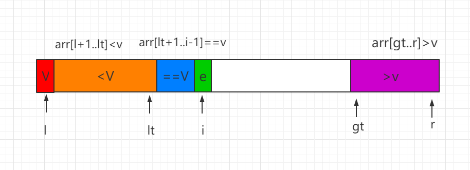
We discuss the partition process in three cases, where i represents the current traversal index position:
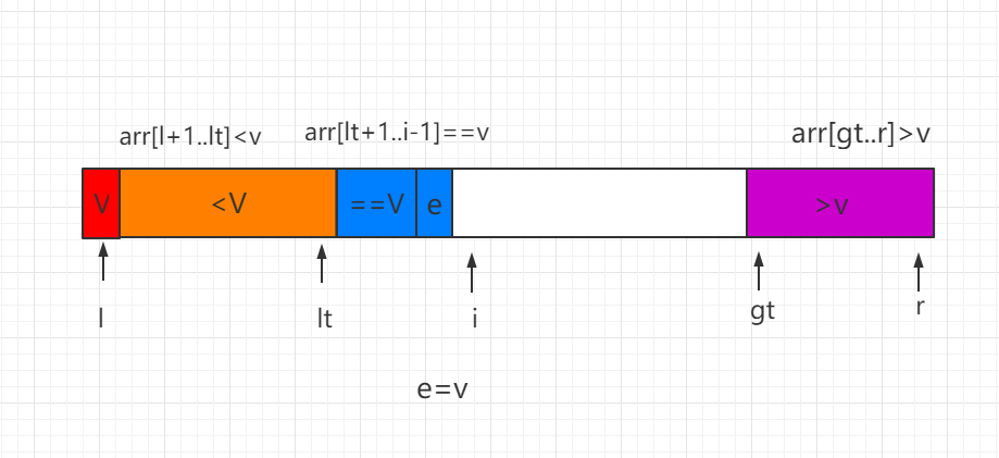
(1) The current element e = V is directly placed into the blue interval, and i moves one position to the right.
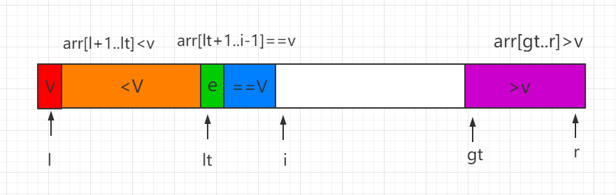
(2) The current element e < v: swap e with the value at the first position of the interval equal to V, and move both lt and i one position to the right.
(3) The current element e > v: swap e with the value at index gt-1, and move the gt index one position to the left.
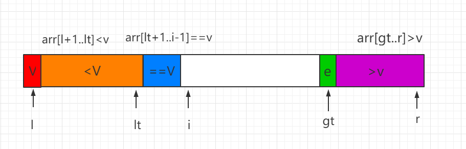
Finally, wheni=gtWhen the traversal ends, swap v with the value pointed to by index lt, and this completes the partitioning process. Then, use the same method to recursively sort the <V and >V parts.
Java example code
Source code package download:Download
QuickSort3Ways.java file code:
/**
* Three-way quick sort
*/
public class QuickSort3Ways {
// Core code --- start
// Recursively use quicksort to sort the range arr[l...r]
private static void sort(Comparable[] arr, int l, int r){
if (l >= r) {
return;
}
// Randomly select a value as the pivot in the range arr[l...r]
swap( arr, l, (int)(Math.random()*(r-l+1)) + l );
Comparable v = arr[l];
int lt = l; // arr[l+1...lt] < v
int gt = r + 1; // arr[gt...r] > v
int i = l+1; // arr[lt+1...i) == v
while( i < gt ){
if( arr[i].compareTo(v) < 0 ){
swap( arr, i, lt+1);
i ++;
lt ++;
}
else if( arr[i].compareTo(v) > 0 ){
swap( arr, i, gt-1);
gt --;
}
else{ // arr[i] == v
i ++;
}
}
swap( arr, l, lt );
sort(arr, l, lt-1);
sort(arr, gt, r);
}
// Core code --- end
public static void sort(Comparable[] arr){
int n = arr.length;
sort(arr, 0, n-1);
}
private static void swap(Object[] arr, int i, int j) {
Object t = arr[i];
arr[i] = arr[j];
arr[j] = t;
}
// Test QuickSort3Ways
public static void main(String[] args) {
// The three-way quick sort algorithm is also an O(nlogn) complexity algorithm
// Can easily handle data on the order of 1 million within 1 second
int N = 1000000;
Integer[] arr = SortTestHelper.generateRandomArray(N, 0, 100000);
sort(arr);
SortTestHelper.printArray(arr);
}
}
Core idea and working principle of the algorithm
The subtlety of the three-way partitioning algorithm is that it uses three pointers to track different regions of the array, completing the three-way classification in a single traversal.
Algorithm partition state
Let's understand the partitioning process of the algorithm through a state diagram:
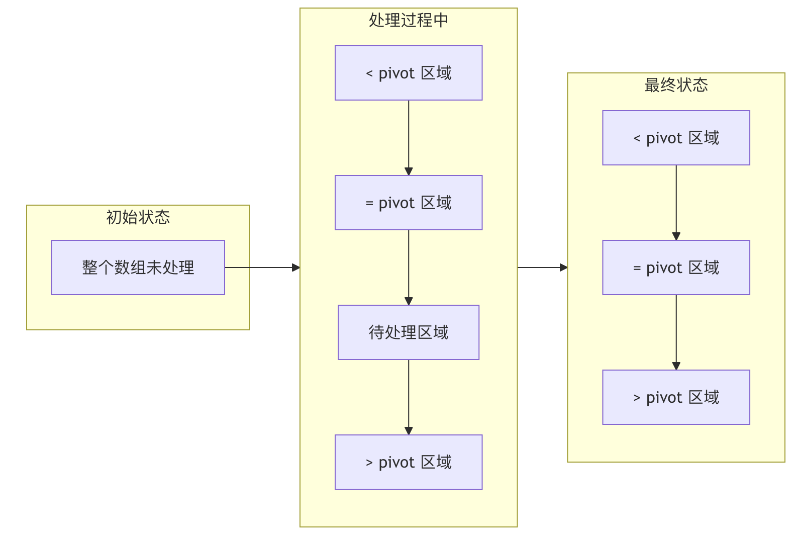
Figure descriptionThe algorithm maintains three pointers (lt, i, gtIt divides the array into four regions; as processing proceeds, the undealt region gradually shrinks, finally forming three clear partitions.
Roles of the three key pointers
lt(less than) pointerPoints to the end of the region less than the pivoti(current) pointerPosition of the element currently being examinedgt(greater than) pointerPoints to the beginning of the region greater than the pivot
Python implementation
Basic three-way partition function
Below is a standard implementation of the three-way partition function; we will analyze it line by line:
Example
"""
Perform three-way partitioning on array arr in the range from low to high
Parameters:
arr: The array to be partitioned
low: The starting index of the partition
high: The ending index of the partition
Returns:
(lt, gt): The left and right boundaries of the region equal to the pivot value
"""
# Choose the pivot (here the first element is chosen)
pivot = arr[low]
# Initialize three pointers
lt = low # The right boundary of the region less than the pivot (initialized to low)
i = low + 1 # Position of the current element being examined
gt = high # The left boundary of the region greater than the pivot (initialized to high)
# Main loop: continue while there are still unprocessed elements
while i <= gt:
if arr[i] < pivot:
# Case 1: The current element is less than the pivot
# Swap it with the next element of the lt pointer to expand the less-than region
arr[lt], arr[i] = arr[i], arr[lt]
lt += 1
i += 1
elif arr[i] > pivot:
# Case 2: The current element is greater than the pivot
# Swap it with the element at the gt pointer to expand the greater-than region
arr[i], arr[gt] = arr[gt], arr[i]
gt -= 1
# Note: i is not incremented here because the swapped-in element has not been examined yet
else:
# Case 3: The current element equals the pivot
# Skip directly, expanding the equal-to region
i += 1
# Return the boundaries of the region equal to the pivot
return lt, gt
Complete three-way quicksort implementation
Based on the partition function above, we can implement the complete three-way quicksort:
Example
"""
Three-way quick sort main function
Parameters:
arr: The array to be sorted
low: The starting index for sorting (default is 0)
high: The ending index for sorting (default is the end of the array)
"""
if high is None:
high = len(arr) - 1
# Recursion termination condition: subarray length is less than or equal to 1
if low >= high:
return
# Perform three-way partitioning
lt, gt = three_way_partition(arr, low, high)
# Recursively sort the part less than the pivot
three_way_quicksort(arr, low, lt - 1)
# Recursively sort the part greater than the pivot
three_way_quicksort(arr, gt + 1, high)
# Note: the part equal to the pivot is already in its correct position, no need to sort further
Practical application examples
Example 1: Color sorting problem
This is a classic application scenario of the three-way partitioning algorithm, also known as the "Dutch National Flag Problem".
Example
"""
Color sorting: arrange an array containing only 0 (red), 1 (white), 2 (blue) in order
Parameters:
colors: The color array, elements are 0, 1, 2
Returns:
The sorted color array
"""
# Initialize three pointers
red_ptr = 0 # The end of the red region
white_ptr = 0 # The current position being examined (also the end of the white region)
blue_ptr = len(colors) - 1 # The beginning of the blue region
while white_ptr <= blue_ptr:
if colors[white_ptr] == 0:
# Red: swap to the red region
colors[red_ptr], colors[white_ptr] = colors[white_ptr], colors[red_ptr]
red_ptr += 1
white_ptr += 1
elif colors[white_ptr] == 1:
# White: remains in the middle region
white_ptr += 1
else:
# Blue: swap to the blue region
colors[white_ptr], colors[blue_ptr] = colors[blue_ptr], colors[white_ptr]
blue_ptr -= 1
# Note: white_ptr is not incremented here because the element swapped in has not been checked yet
return colors
# Test data
test_colors = [2, 0, 2, 1, 1, 0, 1, 2, 0, 1, 0, 2]
print("Original color array:", test_colors)
print("Sorted color array:", sort_colors(test_colors.copy()))
Test data descriptionThe array above represents color codes (0=red, 1=white, 2=blue). After sorting, all zeros should be in front, ones in the middle, and twos at the end.
Example 2: Student score grouping
Suppose we need to segment students by score: below 60 is failing, 60-80 is good, and above 80 is excellent.
Example
"""
Classify the scores into three levels: Fail (<60), Good (60-80), Excellent (>80)
Parameters:
scores: array of scores
Returns:
Segmented scores array
"""
if not scores:
return scores
# Use the three-way partitioning idea, with 60 and 80 as the boundaries
# First partition by 60: Fail vs. Pass or above
low = 0
mid = 0
high = len(scores) - 1
# First round: separate fail scores (<60)
while mid <= high:
if scores[mid] < 60:
scores[low], scores[mid] = scores[mid], scores[low]
low += 1
mid += 1
elif scores[mid] <= 80:
mid += 1
else:
scores[mid], scores[high] = scores[high], scores[mid]
high -= 1
# Second round: separate good and excellent scores from the pass-and-above part
# At this point, low points to the position of the first good score
mid = low
high = len(scores) - 1
while mid <= high:
if scores[mid] <= 80:
mid += 1
else:
scores[mid], scores[high] = scores[high], scores[mid]
high -= 1
return scores
# Test data
test_scores = [45, 78, 92, 56, 85, 67, 72, 88, 59, 95, 61, 73]
print("Original scores:", test_scores)
print("Segmented scores:", categorize_grades(test_scores.copy()))
print("Note: first part <60, middle part 60-80, last part >80")
Algorithm complexity analysis
Time complexity
The time complexity analysis of the three-way sorting algorithm can be expressed with the following formula:
$$ T(n) = O(n) + T(k) + T(n - k - m) $$
Where:
- $n$ is the length of the array
- $k$ is the number of elements less than the pivot value
- $m$ is the number of elements equal to the pivot value
- $n - k - m$ is the number of elements greater than the pivot value
Best caseBest case: Each partition can evenly divide the array into three parts, with time complexity $O(n \log_3 n)$, which is actually still $O(n \log n)$.
Worst caseWorst case: Each partition is extremely unbalanced, with time complexity $O(n^2)$.
Average caseAverage case: For random data, the average time complexity is $O(n \log n)$.
Space complexity
The algorithm is implemented recursively, and the recursion depth depends on the partitioning situation:
- Best case:$O(\log n)$
- Worst case:$O(n)$
Space usage can be reduced through tail recursion optimization or by using an iterative approach.